the x axis ticks does not show when using sf package to plot global map
The X axis ticks does not show when using the geom_sf function of sf package to plot the global map
library(sf)
library(rnaturalearth)
library(stars)
library(ggplot2)
wld <- ne_coastline(returnclass = "sf")
diri <- "https://downloads.psl.noaa.gov/Datasets/ncep.reanalysis.derived/surface/pres.mon.ltm.nc"
da <- read_ncdf(diri, var = "pres") |> units::drop_units()
ds <- da[,,,1] |> as.data.frame()
ds[ds$lon > 180, "lon"] <- ds[ds$lon > 180, "lon"] - 360 # 0°~360° were convert to -180~180°
sf_use_s2(FALSE)
ggplot() +
geom_raster(data = ds, aes(x = lon, y = lat, fill = pres)) +
geom_sf(data = wld) +
coord_sf(expand = FALSE) +
scale_fill_fermenter(palette = "YlOrRd", direction = -1) +
scale_x_continuous(breaks = seq(-135, 135, 45)) +
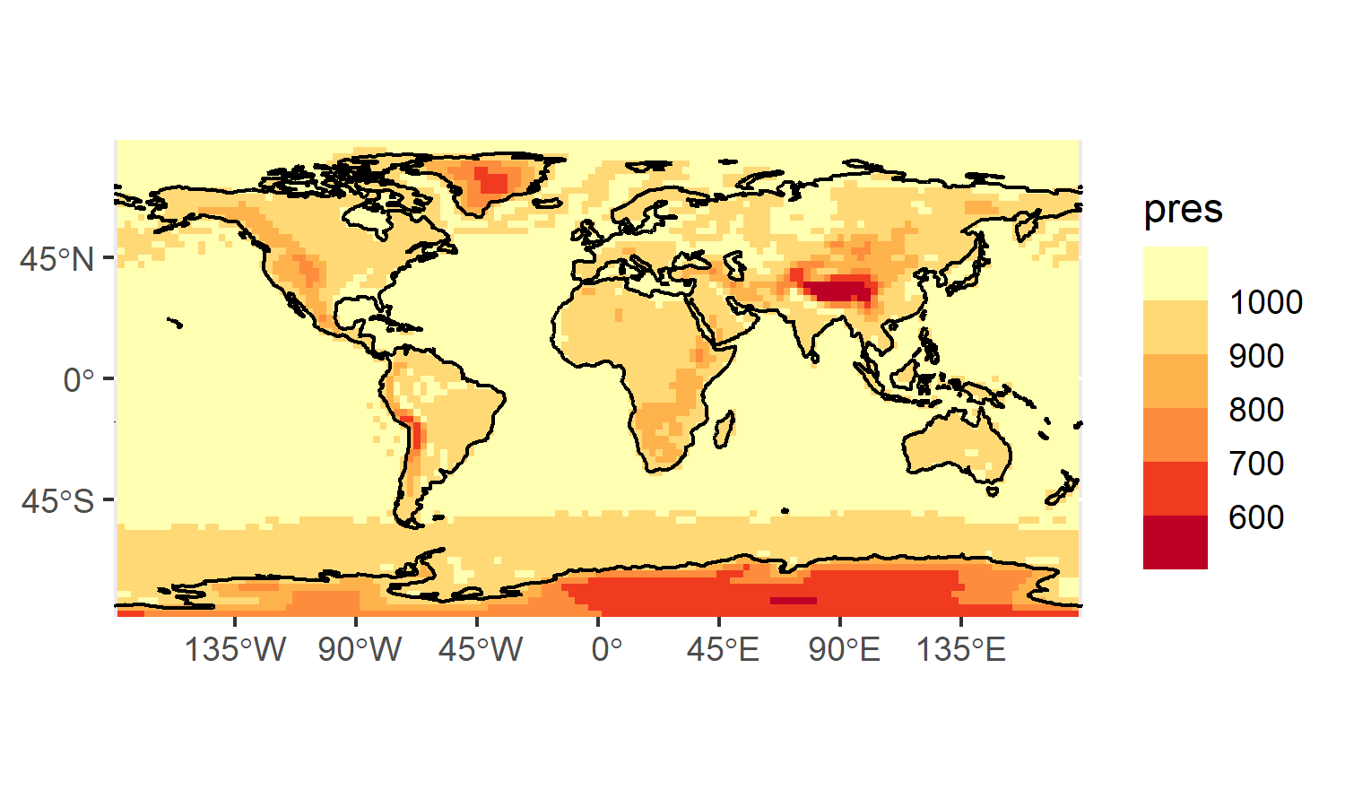
scale_y_continuous(breaks = seq(-45, 45, 45))

as shown in the figure, the X axis ticks does not show at the specified location.
How to solve this problem?
Curious. Slightly simpler reprex (I think we don't need the actual world map to minimally reproduce the problem). I think the root cause is that the raster is technically wrong; it contains the data on lat = -90. A raster's data is not a point, but a tile, which has width and height, so, the data on lat = -90 goes to the area below lat = -90.
But I have no idea why it blows up the ticks...
library(sf)
#> Linking to GEOS 3.9.1, GDAL 3.3.2, PROJ 7.2.1; sf_use_s2() is TRUE
library(rnaturalearth)
library(ggplot2)
library(patchwork)

wld <- ne_coastline(returnclass = "sf")

set.seed(10)
raster <- expand.grid(lon = seq(-180, 180, by = 45), lat = seq(-90, 90, by = 45))
raster$fill <- runif(nrow(raster))

sf_use_s2(FALSE)
#> Spherical geometry (s2) switched off
p1 <- ggplot() +
  geom_sf(data = wld) +
  coord_sf(expand = FALSE) +
  scale_x_continuous(breaks = seq(-135, 135, 45)) +
  scale_y_continuous(breaks = seq(-45, 45, 45)) +
  guides(fill = "none")

# works fine
p1

p2 <- p1 +
  geom_raster(data = raster, aes(x = lon, y = lat, fill = fill), alpha = 0.2)

raster_wo_tail <- raster |> dplyr::filter(lat > -90, lon > -180)
p3 <- p1 +
  geom_raster(data = raster_wo_tail, aes(x = lon, y = lat, fill = fill), alpha = 0.2)

p2 * p3

Created on 2022-04-28 by the reprex package (v2.0.1)
Thank you. The issue was solved using your method.
rm(list = ls())
library(sf)
library(rnaturalearth)
library(stars)
library(ggplot2)
wld <- ne_coastline(returnclass = "sf")
#data_url <- "https://downloads.psl.noaa.gov/Datasets/ncep.reanalysis.derived/surface/pres.mon.ltm.nc"
diri <- "rdata/dataset/pres.mon.ltm.nc"
da <- read_ncdf(diri, var = "pres") |> units::drop_units()
ds <- da[,,,1] |> as.data.frame(xy = TRUE)
ds[ds$lon > 180, "lon"] <- ds[ds$lon > 180, "lon"] - 360   # 0°~360° were convert to -180~180°
ds <- ds[abs(ds$lon) < 180 & abs(ds$lat) < 90, ]
sf_use_s2(FALSE)
ggplot() +
  geom_raster(data = ds, aes(x = lon, y = lat, fill = pres)) +
  geom_sf(data = wld) +
  coord_sf(expand = FALSE) +
  scale_fill_fermenter(palette = "YlOrRd", direction = -1) +
  scale_x_continuous(breaks = seq(-135, 135, 45)) +
  scale_
What blocks the ticks is that the graticule lines don't intersect with the plot boundaries. To draw ticks for any sort of strange, non-linear coordinate system the only reasonable way I could think of to implement it was to look at the intersection points between graticule lines and plot boundaries. This generally places ticks where you would expect them and avoids ticks where they shouldn't be, but it can give you problems for world maps.
The relevant code is here: https://github.com/tidyverse/ggplot2/blob/21df8dc88e9b736a136bc39362defe2943008767/R/coord-sf.R#L316-L471
Thanks. Do you think it's possible to set xlim and ylim automatically on coord_sf()? If possible, I think it would save us.
library(sf)
#> Linking to GEOS 3.9.1, GDAL 3.3.2, PROJ 7.2.1; sf_use_s2() is TRUE
library(rnaturalearth)
library(ggplot2)
library(patchwork)

wld <- ne_coastline(returnclass = "sf")

set.seed(10)
raster <- expand.grid(lon = seq(-180, 180, by = 45), lat = seq(-90, 90, by = 45))
raster$fill <- runif(nrow(raster))

sf_use_s2(FALSE)
#> Spherical geometry (s2) switched off
ggplot() +
  geom_sf(data = wld) +
  coord_sf(
    expand = FALSE,
    xlim = c(-180, 180),
    ylim = c(- 90,  90)
  ) +
  scale_x_continuous(breaks = seq(-135, 135, 45)) +
  scale_y_continuous(breaks = seq( -45,  45, 45)) +
  guides(fill = "none") +
  geom_raster(data = raster, aes(x = lon, y = lat, fill = fill), alpha = 0.2)

Created on 2022-04-29 by the reprex package (v2.0.1)
I would be worried that there are many cases in which it could go wrong, in particular since the limits will depend on the CRS in which the geometries are provided.
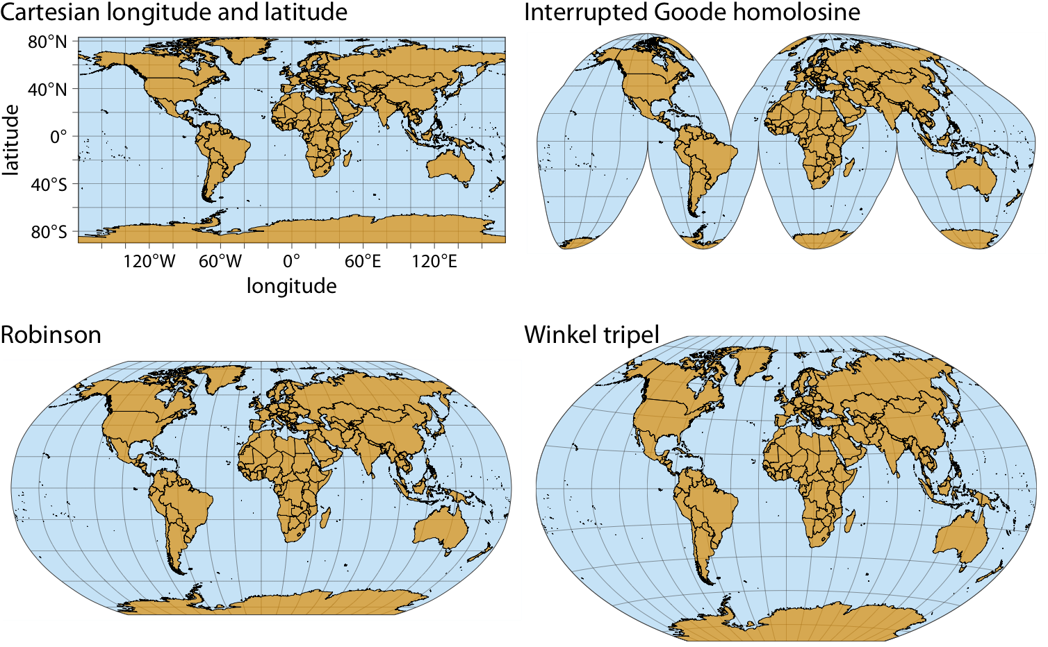
And also, I'd like to point out that when drawing a world map, tick labels only look good when you use a bad projection. The moment you use a reasonable projection (Goode Homolosine or Winkel Tripel) tick labels will be all bunched up near the poles and look weird. In particular for Goode Homolosine.
Maybe the right course of action would be to explain all of this in the documentation?
I see, this makes sense to me. I agree the best option is to explain in the dos.
This issue can also be solved by using this method. Thank you.
rm(list = ls())
library(sf)
library(rnaturalearth)
library(stars)
library(ggplot2)
wld <- ne_coastline(returnclass = "sf")
#data_url <- "https://downloads.psl.noaa.gov/Datasets/ncep.reanalysis.derived/surface/pres.mon.ltm.nc"
diri <- "rdata/dataset/pres.mon.ltm.nc"
da <- read_ncdf(diri, var = "pres") |> units::drop_units()
ds <- da[,,,1] |> as.data.frame(xy = TRUE)
ds[ds$lon > 180, "lon"] <- ds[ds$lon > 180, "lon"] - 360   # 0°~360° were convert to -180~180°
#ds <- ds[abs(ds$lon) < 180 & abs(ds$lat) < 90, ]
sf_use_s2(FALSE)
ggplot() +
  geom_raster(data = ds, aes(x = lon, y = lat, fill = pres)) +
  #geom_stars(data = ds) +
  geom_sf(data = wld) +
  coord_sf(expand = FALSE,
           xlim = c(-180, 180),
           ylim = c(- 90,  90)) +
  scale_fill_fermenter(palette = "YlOrRd", direction = -1) +
  scale_x_continuous(breaks = seq(-135, 135, 45)) +
  scale_y_continuous(breaks = seq(-45, 45, 45)) +
  theme(axis.title = element_blank())
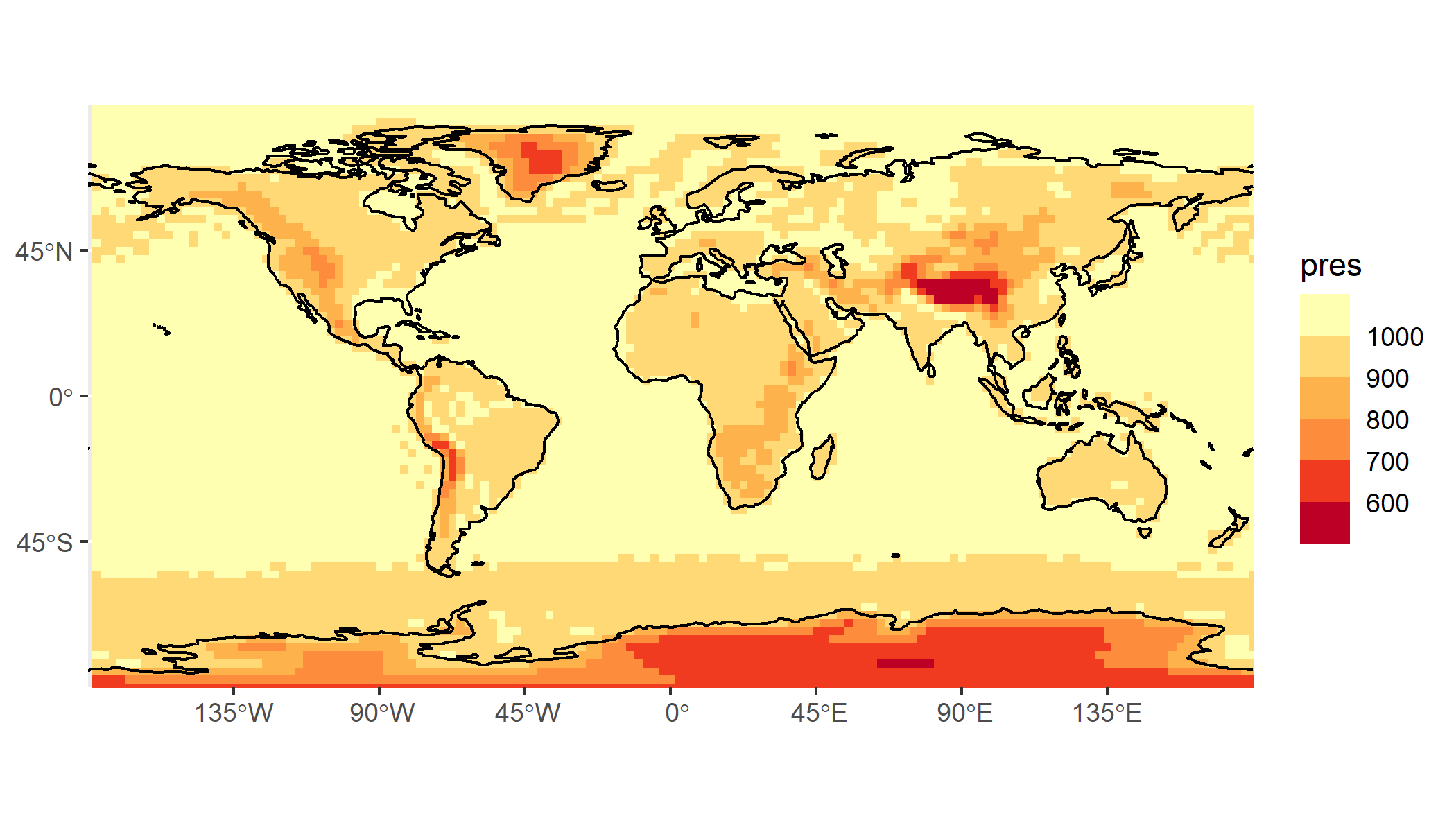
What blocks the ticks is that the graticule lines don't intersect with the plot boundaries. To draw ticks for any sort of strange, non-linear coordinate system the only reasonable way I could think of to implement it was to look at the intersection points between graticule lines and plot boundaries. This generally places ticks where you would expect them and avoids ticks where they shouldn't be, but it can give you problems for world maps.
The relevant code is here:
https://github.com/tidyverse/ggplot2/blob/21df8dc88e9b736a136bc39362defe2943008767/R/coord-sf.R#L316-L471
Thank you.
I would be worried that there are many cases in which it could go wrong, in particular since the limits will depend on the CRS in which the geometries are provided.
And also, I'd like to point out that when drawing a world map, tick labels only look good when you use a bad projection. The moment you use a reasonable projection (Goode Homolosine or Winkel Tripel) tick labels will be all bunched up near the poles and look weird. In particular for Goode Homolosine.
Maybe the right course of action would be to explain all of this in the documentation?
Yes, I also have all kinds of problems when drawing maps using sf and ggplot2, and sometimes I enen want to use the cartopy package of Python.
I think we discussed this before, but would it make sense to provide an annotation helper that places tick labels inside the plotting are for all these world-map edge cases?
In my opinion this is a good idea in principle but not at all easy to implement, and you may create all sorts of additional expectations by providing this feature. It would probably fit better into a package such as ggspatial.
Simplest reprex for this problem, solved here setting expand=FALSE.
If one were to summarise this issue, is it correct to say that when x/y axis do not show up, one should use coord_sf(expand = FALSE) (given that manual corrections with scale_y_continuous() and scale_x_continuous() are not guaranteed to produce an axis without expand = FALSE?
library(ggplot2)
library(rnaturalearth)

world <- ne_countries(scale = "medium", returnclass = "sf")
p <- ggplot(data = world) +
  geom_sf()

p

p+coord_sf(expand = FALSE)

## manual corrections sometime work without setting explcitly `expand = FALSE`
p+scale_y_continuous(limits = c(-70, 80))+scale_x_continuous(limits = c(-180, 180))

Created on 2023-05-28 with reprex v2.0.2