new interpolation scheme

[pgree]

Edit: Rendered version here

I've added an interpolation function in this pull request https://github.com/stan-dev/math/pull/1814

@bbbales2 alerted me to the need for this sort of interpolation, but there are lots of judgement calls on the way in terms of algorithm and implementation.

@bgoodri mentioned that there might be some relevant interpolation schemes in upcoming Boost releases.

@bob-carpenter has commented on other interpolation issues and discourse discussions in the past.

[pgree]

@bgoodri @wds15

@bbbales2 and I were hoping to get your thoughts on an interpolation algorithm for which I just made a pull request here https://github.com/stan-dev/math/pull/1814.

@bbbales2 mentioned that the need for interpolation has come up in a few places in math issues and discourse discussions. Ben and I chatted about what would make sense. We settled on what's basically linear interpolation with some Gaussian smoothing (and shifting so that the interpolated points intersect the reference points). As a bonus, the interpolated function and its derivative are basically analytic.

Here's a simple example of how that looks:

[bgoodri]

Haven't looked at it but there is all kinds of stuff in Boost

https://www.boost.org/doc/libs/1_72_0/libs/math/doc/html/interpolation.html

On Fri, Apr 3, 2020 at 4:31 PM pgree [email protected] wrote:

@bgoodri https://github.com/bgoodri @wds15 https://github.com/wds15

@bbbales2 https://github.com/bbbales2 and I were hoping to get your thoughts on an interpolation algorithm for which I just made a pull request here stan-dev/math#1814 https://github.com/stan-dev/math/pull/1814.

@bbbales2 https://github.com/bbbales2 mentioned that the need for interpolation has come up in a few places in math issues and discourse discussions. Ben and I chatted about what would make sense. We settled on what's basically linear interpolation with some Gaussian smoothing (and shifting so that the interpolated points intersect the reference points). As a bonus, the interpolated function and its derivative are basically analytic.

Here's a simple example of how that looks: [image: Screen Shot 2020-04-03 at 4 20 50 PM] https://user-images.githubusercontent.com/61166344/78401747-6fa13900-75c7-11ea-8c83-214f3de2fc95.png

— You are receiving this because you were mentioned. Reply to this email directly, view it on GitHub https://github.com/stan-dev/design-docs/pull/18#issuecomment-608644551, or unsubscribe https://github.com/notifications/unsubscribe-auth/AAZ2XKQIN2G5Z2BPR2M5GPDRKZBTJANCNFSM4LZBH4AQ .

[bob-carpenter]

@betanalpha may also have useful input. At some point, you wind up building spline models and then GPs. So the question in my mind is how elaborate to make a simple interpolation function.

For comparison, here's the interpolation function in BUGS and JAGS:

interp.lin(u, xs, ys) = ys[n] + p * (ys[n+1] - ys[n])

where

• u is a scalar,
• xs and ys are the same size vectors,
• xs is sorted in ascending order,
• xs[n] <= u < xs[n + 1], and
• p = (u - xs[n]) / (x[n + 1] - x[n]).

So it's not differentiable at points in xs, nor is it defined outside of (xs[1], xs[N]) where N = size(xs).

So the question is what the extra smoothness is going to buy us on the algorithm side?

[andrewgelman]

At the very least, I'd extend to f(x) = f(x_1) below the minimum value and f(x) = f(x_N) above the maximum value (or, if we go with some smoother curve, an equivalent sort of extrapolation). I don't want to overthink this one: an extrapolation is just an extrapolation; it generally won't be right and we don't want to pretend otherwise. But a null extrapolation can come in handy. It comes up from time to time, and it's always a pain to do this extension "manually."

On Apr 3, 2020, at 5:09 PM, Bob Carpenter [email protected] wrote:

@betanalpha https://github.com/betanalpha may also have useful input. At some point, you wind up building spline models and then GPs. So the question in my mind is how elaborate to make a simple interpolation function.

For comparison, here's the interpolation function in BUGS and JAGS:

interp.lin(u, xs, ys) = ys[n] + p * (ys[n+1] - ys[n])

where

u is a scalar, xs and ys are the same size vectors, xs is sorted in ascending order, xs[n] <= u < xs[n + 1], and p = (u - xs[n]) / (x[n + 1] - x[n]). So it's not differentiable at points in xs, nor is it defined outside of (xs[1], xs[N]) where N = size(xs).

So the question is what the extra smoothness is going to buy us on the algorithm side?

— You are receiving this because you are subscribed to this thread. Reply to this email directly, view it on GitHub https://github.com/stan-dev/design-docs/pull/18#issuecomment-608667453, or unsubscribe https://github.com/notifications/unsubscribe-auth/AAZYCUM2H2DNIFXJVFBILATRKZGBXANCNFSM4LZBH4AQ.

[betanalpha]

“Yes-anding” Bob’s comment I do not think that any deterministic interpolation scheme is a good idea for Stan because there is no unique way to interpolate and interpolation as a deterministic process is ill-posed. Interpolation is fundamentally an inference problem — we have finite data and maybe some constraints like smoothness implicit coded in the interpolation model. There will always be an infinite number of ways to satisfy these constraints and so reporting just one will always be underestimating the uncertainty inherent to the problem. Giving users access to a single interpolator within the Stan language will just give them easy ways to build bad models.

Were interpolation this easy people would spend their careers on splines and GPs which are nothing but interpolation with uncertainty!

On Apr 3, 2020, at 5:09 PM, Bob Carpenter [email protected] wrote:

@betanalpha https://github.com/betanalpha may also have useful input. At some point, you wind up building spline models and then GPs. So the question in my mind is how elaborate to make a simple interpolation function.

For comparison, here's the interpolation function in BUGS and JAGS:

interp.lin(u, xs, ys) = ys[n] + p * (ys[n+1] - ys[n])

where

u is a scalar, xs and ys are the same size vectors, xs is sorted in ascending order, xs[n] <= u < xs[n + 1], and p = (u - xs[n]) / (x[n + 1] - x[n]). So it's not differentiable at points in xs, nor is it defined outside of (xs[1], xs[N]) where N = size(xs).

So the question is what the extra smoothness is going to buy us on the algorithm side?

— You are receiving this because you were mentioned. Reply to this email directly, view it on GitHub https://github.com/stan-dev/design-docs/pull/18#issuecomment-608667453, or unsubscribe https://github.com/notifications/unsubscribe-auth/AALU3FTHY7A2X6W7RGCLEPTRKZGBXANCNFSM4LZBH4AQ.

[bob-carpenter]

@betanalpha --- I wasn't trying to say this was a bad idea. I think for any tool we provide it's easy to say that something more sophisticated should be used.

So my question was really (a) do we just do simple interpolation and leave the data points non-differentiable, or (b) do we do something like this?

Edit: Also, I understand the part about uncertainty, but we also do this all the time. A linear regression is deterministic and an ODE's just a fancier version of a deterministic interpolation subject to some side conditions. We can put errors on top of this if we need to. But I do agree it's hard to imagine a generative model where this is something you'd use. I suspect that's why it's not already in Stan.

[pgree]

Thanks for all the comments. We decided to implement a scheme in which the interpolated function is differentiable based on several comments/requests on discourse and github:

https://discourse.mc-stan.org/t/linear-interpolation-and-searchsorted-in-stan/13318/1 https://discourse.mc-stan.org/t/vectors-arrays-interpolation-other-things/10253/17 https://github.com/stan-dev/stan/issues/1165 https://github.com/stan-dev/stan/issues/1214 https://github.com/stan-dev/math/issues/58

@avehtari might also be interested as he has commented in discourse on interpolation.

[betanalpha]

Edit: Also, I understand the part about uncertainty, but we also do this all the time. A linear regression is deterministic and an ODE's just a fancier version of a deterministic interpolation subject to some side conditions. We can put errors on top of this if we need to. But I do agree it's hard to imagine a generative model where this is something you'd use. I suspect that's why it's not already in Stan.

Right. To me interpolation is a 100% a modeling problem, not something that can be solved with a new function. The ambiguity of possible interpolation schemes just reinforces the fact that this isn't something that can be solved deterministically. We already have a wide range of possible interpolation models, including GPs and splines, so what does this offer other than making it easy for users to ignore the inferential need?

[wds15]

It's great to see progress in this regard. I do think that we really need something like this. While I agree in that interpolation is an inference problem in many cases, there are a good deal of applications where we condition on some input function - for example on the dosing history in PK/PD problems.

I would welcome if we would have interpolation functions of varying complexity. Simple first:

• last observation carry forward (constant between successive values)
• linear interpolation
• something smoothed as you are suggesting

While I would appreciate all of them being done at once, I don't want to put this on you (unless you want to). However, please make a proposal as to how such functions would like consistently. We would like to have a common and meaningful syntax for them.

Now, for the smoothing flavours, I would find it important to give users control over (easy) tuning parameters for the smoothness. It's hard for me to see that the smoothing is universally correct for every application.

As I would attempt to use this type of functions as forcing functions to ODEs, I would very much appreciate that these functions are fast. Hearing that you call an error function does not sound like it is very fast. Recall that for ODE solvers this function will get called many times. Maybe requiring sorted inputs and all that will also help you to speed up things?

Now, for the documentation of all of this, it would be great if you could advise users as to how they can minimise the amount of data needed to pass into the interpolation function while maintaining good accuracy in representing the to-be approximated function.

I hope this helps; please let me know if some points are not clear enough.

(for PK/PD problems in particular it would be awesome to super-impose a series of exponentials directly... just to spark your creativity...)

[bbbales2]

So the question is what the extra smoothness is going to buy us on the algorithm side?

I think HMC requires one derivative for the stats math to work. Leapfrog integrator takes two derivatives to keep its second order error (which I assume is important cuz there's a pretty big difference between first and second order methods).

Given we control what goes in, I would like to keep both of those derivatives.

At some point, you wind up building spline models and then GPs

I don't think that's always true even in a statistics sense. Sometimes you'd do some sorta random process, and sometimes you'd just give up and fit a line.

do we just do simple interpolation and leave the data points non-differentiable

In @bob-carpenter 's notation, I think the easiest is u is differentiable and xs and ys are data.

There will always be an infinite number of ways to satisfy these constraints and so reporting just one will always be underestimating the uncertainty inherent to the problem

This argument works for everything in the model. Why normal instead of something else, why logistic link, etc.

To me interpolation is a 100% a modeling problem

True, but I think it's like measurement error models -- everything could be a measurement error model but most of the time we just pretend a measurement 3.4 means 3.4000000000000... and roll with it. Same here -- something got fit or measured somewhere else and the knowledge is encoded as a lookup table, so just condition on that. We assuming ignoring this uncertainty isn't gonna hurt us. sqrt(5^2 + 12^2) = 13, etc.

---

Re: algorithms,

1. I don't like piecewise constant. Those discontinuities could really mess up the sampler. I could see how if this was a forcing function in an ODE the output could still be differentiable, but ODE solvers don't like those steps either.

2. People do piecewise linear now. I suspect they'd do cubic splines or whatever we gave them. I think interpolation is something people do out of convenience than anything.

3. I suspect if we required sorted inputs, we'd get bugs. Maybe if we checked every time we did a lookup for out-of-order things we'd catch errors, but it still seems finicky.

For N data points, linear/cubic interpolation would be O(N) algorithms if we checked sorting every time, and O(logn) without, so the second seems attractive, but it is nice to have functions that are super safe about stuff.

Doing GP interpolation and just taking the mean would require an O(N^3) solve in transformed data and then some O(N) dot product evaluations. The advantage there is that the sort isn't necessary and a a dot product is easier (though the complexity is the same).

If we vectorize these functions, the linear/cubic interpolations can amortize the order checks. The GP complexity remains the same. In the ODE use case though we don't get to vectorize though.

I guess what's the complexity of the algorithm in https://github.com/stan-dev/math/pull/1814 ?

[bob-carpenter]

People do piecewise linear now. I suspect they'd do cubic splines or whatever we gave them.

I agree. I think it just comes down to efficiency in the HMC context.

I think the easiest is u is differentiable and xs and ys are data

We should make everything differentiable if it's just an ordinary Stan program.

I suspect if we required sorted inputs, we'd get bugs.

That matches what BUGS did. Without the sorting, we have to walk over the entire input array instead of using binary search. And if we allowed a vector of prediction inputs we'd want to do the sorting for efficiency internally.

I think HMC requires one derivative for the stats math to work.

Because of broken reversibility? The thing is that the curve around the interpolated points has to big enough to matter because otherwise it's going to work just like having a non-differentiable point in terms of divergence.

[pgree]

We should make everything differentiable if it's just an ordinary Stan program.

I will look into this. Right now, the codes only provide derivatives of f(t) with respect to t where f is the interpolated function.

I would find it important to give users control over (easy) tuning parameters for the smoothness

We can include an input in the interpolation function that corresponds to how much smoothing the user wants. For example, the input could be a number on the interval [0, 1] where 0 corresponds to linear interpolation and 1 is a very smooth interpolation. Do you think that would be enough user control over smoothing?

I would very much appreciate that these functions are fast. Hearing that you call an error function does not sound like it is very fast

It shouldn't be a problem to speed up the evaluation of the error function if it's not fast right now.

it would be great if you could advise users as to how they can minimise the amount of data needed to pass into the interpolation function while maintaining good accuracy

Sounds good, will do.

I guess what's the complexity of the algorithm in stan-dev/math#1814 ?

Under reasonable conditions, it's O(n + k*log(n)) where n is the number of points in the function tabulation and k is the length of the sorted vector of points at which the user wants to evaluate the interpolated function. How big do you reasonably expect k and n to be in practice? The constant could dominate for small k and n.

[wds15]

I don't quite see as to why everything must be differentiable - as long as things are data everything is fine.

Things which can be cast to a var aka a parameter should always stay differentiable, of course.

Yet, we do condition in our models on the covariates "X" most of the time without modelling this space.

In that sense last observation carry forward or linear interpolation are fine ways of interpolating to me at least.

[bbbales2]

For example, the input could be a number on the interval [0, 1] where 0 corresponds to linear interpolation and 1 is a very smooth interpolation. Do you think that would be enough user control over smoothing?

I know how to interpret 0 there, but I don't know how to interpret 1.

Somehow it needs to be possible for people to check what they're doing. expose_stan_functions is one way, but that's not available for cmdstan users.

If someone is putting an interpolation in their model, somewhere in their workflow they need to check if it's doing the right thing.

How big do you reasonably expect k and n to be in practice

Just making up numbers, I think the most common k would be 1, and n would be in the 10-100 range. (Edit: and I'm making these numbers up because I think this would be useful for implementing lookup-table functions -- not interpolating through a big cloud of points with where n might conceivably be much higher and the interpolant doesn't closely track the reference points).

In that sense last observation carry forward or linear interpolation are fine ways of interpolating to me at least.

differentiability of u so it can be a parameter would be convenient. I don't think xs or ys are gonna be worth the effort (and it'd screw up performance of interpolating with a GP mean -- O(N^3) complexity even if it were possible).

[bob-carpenter]

I don't quite see as to why everything must be differentiable - as long as things are data everything is fine.

We could put data qualifiers in front of arguments. But why do that if we don't have to?

Yet, we do condition in our models on the covariates "X" most of the time without modelling this space.

The point is just that if I write normal_lpdf(y | x * beta, sigma), any of y, x, beta, sigmacan be a variable. It's just a mdoeling choice to use constantx`. Same goes for our linear regression glm function.

It's no big deal if it's too hard to make these differentiable. We just have to be very careful to document that with data qualifiers.

[bob-carpenter]

input could be a number on the interval [0, 1] where 0 corresponds to linear interpolation and 1 is a very smooth interpolation.

Did you mean smoothness or regularization? Something like a Matern covariance matrix for a GP has a parameter that determines order of differentiability, which seems like a natural way to control smoothness in the differentiability sense. But if you mean regularization, that's more like the kind of bandwidth control you get in kernel smoothers where the limit is something like a straight line.

[pgree]

Did you mean smoothness or regularization?

By smoothness I meant the size of the standard deviation in the Gaussian kernel in the convolution.

I know how to interpret 0 there, but I don't know how to interpret 1.

One idea is we could impose a maximum on the standard deviation in the kernel. For example, we could set the maximum standard deviation to be 1/3 the smallest distance between successive points. There are certainly issues that could come up with this approach, and it might not be very clear to the user what's happening without reading a lot of documentation.

Does anyone have thoughts on how to include a smoothness parameter that isn't confusing to the user? Or how important it is to have such a parameter?

[bbbales2]

For example, we could set the maximum standard deviation to be 1/3 the smallest distance between successive points.

This seems to be more attached to if the interpolation goes through all the data points or not? Would there be a way to write smoothness in terms of maximum error from any data point? That sounds like something that would have to be computed beforehand.

Does anyone have thoughts on how to include a smoothness parameter that isn't confusing to the user?

The options are (I'll annotate downsides, upsides as I understand them):

1. Piecewise constant - Not differentiable in a way that'd probably mess up NUTS if u was parameter. O(K logN) assuming inputs sorted

2. Piecewise linear - It's what people are using. Not differentiable in u. Fast. O(K logN) assuming inputs sorted.

3. Cubic spline - Has a derivative in u. Fast. Probably interpolates badly with non-uniform points. O(K logN) assuming inputs sorted

4. Boost interpolants - Probably has derivatives in u. Boost handles testing/maintenance. Seems to advertise working for periodic functions, non-uniformly spaced points, etc. Varies.

5. The Gaussian convolution thing - Has (lots of?) derivatives in u. Requires setting smoothing parameter. O(N + k logN)

6. Expectation of GP - Might have derivatives in u? I'm just assuming it does lol. Requires O(N^3) computation beforehand. Two smoothing parameters to set for RBF kernel. O(KN)

--

Other things:

It seems weird to talk about interpolation but not talk about error. I suspect the types of interpolations people are doing are writing down points off a plot in a paper and calling it a day. I don't think people are doing interpolations that need to be accurate to 1e-8 though.

I don't think an interpolation utility in Stan is something for automatically interpolating a cloud of points. Like, I think we should design this to operate in the realm where we expect to go through all the points. Line going through a cloud of points is the more-statistics problem and we aren't really trying to solve that here.

Regarding @andrewgelman's comment about extrapolation

1. Do we handle that automatically in some way?

2. Do we accept xs at -inf and +inf?

3. Do we have a switch for this behavior?

Edit: Also it seems clear that people either need a way to reproduce the interpolation outside of Stan so that they can know what they're actually doing inside Stan. I guess this is what expose_stan_functions does. What are the other options for each thing, I guess.

[andrewgelman]

I put in a vote for piecewise linear, at least as one of the options. I say this first because it's quick and transparent, second because I've done this linear interpolation a few times, and it's kind of a pain in the ass to do it by hand. I also vote for extending x_1 at the low end and x_N at the high end.

For what it's worth, I was never seeing this interpolation thing as a data smoother or as a statistical model; to me, it's always just been a math function. To put it another way, I was never thinking of using the interpolator as a model for "y"; I was always thinking about it as being for "x".

It's just something that comes up often enough in applications, for example we have data from a bunch of years and we're adjusting to the census, but we only have the census every 10 years. A real model would be better, but as a researcher/modeler, I have to pick my battles!

I was never imagining the interpolator as something to fit to a cloud of points. But who knows, maybe it's a good idea? As in many cases, a generalization that may seem inappropriate can still be useful.

Andrew

On Apr 7, 2020, at 4:36 PM, Ben Bales [email protected] wrote:

For example, we could set the maximum standard deviation to be 1/3 the smallest distance between successive points.

This seems to be more attached to if the interpolation goes through all the data points or not? Would there be a way to write smoothness in terms of maximum error from any data point? That sounds like something that would have to be computed beforehand.

Does anyone have thoughts on how to include a smoothness parameter that isn't confusing to the user?

The options are (I'll annotate downsides, upsides as I understand them):

Piecewise constant - Not differentiable in a way that'd probably mess up NUTS if u was parameter. O(K logN) assuming inputs sorted

Piecewise linear - It's what people are using. Not differentiable in u. Fast. O(K logN) assuming inputs sorted.

Cubic spline - Has a derivative in u. Fast. Probably interpolates badly with non-uniform points. O(K logN) assuming inputs sorted

Boost interpolants - Probably has derivatives in u. Boost handles testing/maintenance. Seems to advertise working for periodic functions, non-uniformly spaced points, etc. Varies.

The Gaussian convolution thing - Has (lots of?) derivatives in u. Requires setting smoothing parameter. O(N + k logN)

Expectation of GP - Might have derivatives in u? I'm just assuming it does lol. Requires O(N^3) computation beforehand. Two smoothing parameters to set for RBF kernel. O(KN)

--

Other things:

It seems weird to talk about interpolation but not talk about error. I suspect the types of interpolations people are doing are writing down points off a plot in a paper and calling it a day. I don't think people are doing interpolations that need to be accurate to 1e-8 though.

I don't think an interpolation utility in Stan is something for automatically interpolating a cloud of points. Like, I think we should design this to operate in the realm where we expect to go through all the points. Line going through a cloud of points is the more-statistics problem and we aren't really trying to solve that here.

Regarding @andrewgelman https://github.com/andrewgelman's comment about extrapolation

Do we handle that automatically in some way?

Do we accept xs at -inf and +inf?

Do we have a switch for this behavior?

— You are receiving this because you were mentioned. Reply to this email directly, view it on GitHub https://github.com/stan-dev/design-docs/pull/18#issuecomment-610607485, or unsubscribe https://github.com/notifications/unsubscribe-auth/AAZYCUIWD6DDZFAUZVPHLQTRLOFFXANCNFSM4LZBH4AQ.

[betanalpha]

I don't think that's always true even in a statistics sense. Sometimes you'd do some sorta random process, and sometimes you'd just give up and fit a line.

This argument works for everything in the model. Why normal instead of something else, why logistic link, etc.

These are not correct analogies to the proposed interpolation. In all of those cases one is imposing assumptions to define a model pi(data | parameters) * pi(parameters) that captures many possible configurations and then conditioning on the data to infer them. Even the most degenerate limit, where there is only a single model configuration that is indifferent to the observed data, is not comparable to the proposed interpolation.

The proposed interpolation rather uses the data to inform the structure of the model itself before any inference is performed, implicitly introducing a form of empirical Bayes that is fundamentally different to any purely generative model.

I think HMC requires one derivative for the stats math to work. Leapfrog integrator takes two derivatives to keep its second order error (which I assume is important cuz there's a pretty big difference between first and second order methods).

Because of broken reversibility? The thing is that the curve around the interpolated points has to big enough to matter because otherwise it's going to work just like having a non-differentiable point in terms of divergence.

Neither of these statements are true. I find it incredibly frustrating when arguments like this are based on speculation about the algorithms.

For all intents and purposes the interpolation would have to be smooth (infinite derivatives) to avoid compromising shadow Hamiltonian systems and hence the scalability of symplectic integrators.

Yet, we do condition in our models on the covariates "X" most of the time without modelling this space.

Because in regression one assumes that the distribution of the covariates is ignorable if we only want to infer the conditional behavior of y given the observed covariates,

pi(y, x | theta) = pi(y | x, theta) * pi(x | theta) = pi(y | x, theta) * pi(x) \propto pi(y | x, theta).

In order to condition on unobserved covariates one has to model pi(x) as it is no longer ignorable. Imposing a fixed interpolation presumes a delta function around some particular interpolation while a data-dependent interpolation implicitly introduces empirical Bayes.

[pgree]

I've updated the Guide-Level Explanation section of the design doc here with a couple of Stan code snippets showing possible implementations of linear interpolation and smooth interpolation.

@andrewgelman for the linear interpolation we will extend x_1 at the low end and x_N at the high end

@wds15 - the example I just added to the design doc uses interpolation in the context of ODE solves, so I would be curious to get your thoughts on this. I haven't included in this version a couple of features you mentioned above including the tuning parameter for smoothness.

[nhuurre]

I'm not a fan of this Gaussian convolution scheme which seems too complicated. I don't think users want to fiddle with a smoothing parameter.

While piecewise linear interpolation is very attractive due to its simplicity it has the disadvantage that it interacts poorly with Stan's gradient-based algorithms.

As an alternative, here's an efficient and easy to understand scheme that can have as many derivatives as needed. The green curve interpolates the black dots: It's constructed as follows: Any three consecutive points define a second degree polynomial. These form the quadratic envelope. The interpolant is weighted average of the two quadratics where the weight depends on the relative distance to the points the quadratics are centered on. In the above picture the weight function is simply

w(t) = 1 - t

The weight function could be any strictly decreasing smooth function with w(0)=1 and w(1)=0. If the first N derivatives of the weight function vanish at both endpoints then the resulting interpolant has N+1 continuous derivatives. So the above choice gives a piecewise cubic polynomial interpolant that has one continuous derivative. It is basically cubic Hermite interpolation.

Trying to increase the differentiability naturally leads one to consider the weight function

w(t) = 1 - 3t^2 + 2t^3

which gives a piecewise quintic polynomial with two continuous derivatives.

Finally, going all the way to infinitely-differentiable, one option is

w(t) = 1/(1 + exp(1/(1-t) - 1/t))

Regardless of the weight function, the quadratic envelope restricts the interpolant to behave in a somewhat predictable fashion. The interpolant depends only on the four nearest points and if they are collinear (or on the same parabola) the line (or parabola) is recovered exactly. It can still oscillate when the distances between data points are very uneven. Still, one can probably control the oscillations by adding a few more points, perhaps using some interpolation available outside of Stan.

Smooth interpolation of the black points, optionally augmented with red dots to remove excessive bumps.

BONUS: So, I was curious just how much smoothness does HMC require. I did a simplistic numerical experiment to measure the energy nonconservation which is a proxy for how much the Metropolis acceptance probability drops every time the integrator walks over a discontinuity.

The idea is to use the leapfrog integrator to simulate a 1D particle hitting a barrier of constant force and observe its energy after it bounces back.

The potential energy is interpolated using the various alternatives described in this post. No Gaussian convolution though because my attempted Python implementation had too many bugs. For comparison there's also the analytic function log1p_exp(2x)/2 which does not go through the points but creates a similar corner in the potential. Cubic, quintic, and smooth are prety much indistinguishable in the upper plot. Their derivatives in the lower plot are still distinct.

The particle has mass 10 and incoming momentum 10 so speed is 1 and the distance traveled per timestep before hitting the barrier is numerically equal to step size. It has enough kinetic energy to move past the interpolated corner deep into the constant-force region where it finally slows and turns around. The kinetic energy is observed again after it has left the barrier.

Here's the plot of the energy difference as a function of the integrator's stepsize.

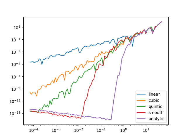
With a large stepsize the particle simply skips over the corner region and every potential looks the same.

Below the critical stepsize of about 0.2 the motion in the analytic potential is fully controlled by a shadow Hamiltonian and only floating point errors contribute to energy noncoservation. Smaller stepsize requires taking more steps and consequently more floating point errors.

The plot seems to suggest that a discontinuity in nth derivative causes energy error of size O(e^n).

[avehtari]

@nhuurre, excellent illustration!

[wds15]

Thanks a lot for the ODE example - this is exactly what I would like to be doing.

Some thoughts from my end here: We should settle on a system how we name these functions and what the argument structure should look like. My preference would be to with something like

interpolate_algo(x, x-data, y-data, ... morge arguments ....)

Feel free to modify - but please lay out a system like this which will be make it possible to add in the future in the same logic another algorithm. We will definitely extend in the future interpolation schemes as there are many available.

What I would encourage in doing is to force the x-data, y-data and the tuning parameters of the algorithm to be data in Stan. This decision should be documented in the design doc. Deviations from it should be done cautiously, I think.

Another consideration I would like to see at least discussed, is the need for ordering of the x-space. I would require an ordering of the x-data to ensure that you can do things like binary search (another input could be x-deltas and a x0 while enforcing positive x-deltas, but maybe that's confusing).

While I agree in that we should not provide foot guns to our users, we should still be open to simple things. After all we also provide a max function to users, so that I don't think that it is needed to put linear interpolation schemes of the table here.

@nhuurre Your suggested interpolation scheme looks very nice. I feel very much reminded of my physics courses years back. Nice.

[pgree]

@nhuurre - thanks for the numerical experiments and the interpolation scheme. One environment in which the Gaussian-smoothed interpolation can come in handy is when you have a smooth function tabulated at enough points such that in between points, the function is well-approximated by a line. Using quadratics/cubics can lead to undesired behavior in between points, like bumps.

Feel free to modify - but please lay out a system like this which will be make it possible to add in the future in the same logic another algorithm.

Good idea, will do.

What I would encourage in doing is to force the x-data, y-data and the tuning parameters of the algorithm to be data in Stan.

Another consideration I would like to see at least discussed, is the need for ordering of the x-space. I would require an ordering of the x-data

These both sound good to me.

[dmi3kno]

@nhuurre quadratic envelope in tidyverse

library(tidyverse)
dat <- tibble(
  x=c(1, 2, 3, 4),
  y=c(0.5, 0.8, 0.15, 0.72),
  i=x) 

dat_i <- tibble(x_pred=runif(50, min(dat$x), max(dat$x)),
                y_pred=NA_real_,
                i=x_pred)

d <- dat %>% 
  mutate(xs=pmap(list(lag(x), x, lead(x)), c),
         ys=pmap(list(lag(y), y, lead(y)), c),
         xsm=map(xs, ~outer(.x, seq(0,2), `^`))) %>% 
  head(-1) %>% tail(-1) %>% 
  mutate(v=map2(xsm, ys, ~solve(.x, .y))) %>% 
  select(x, v)

w <- function(t) 
  1/(1 + exp(1/(1-t) - 1/t))
  #1 - t
  #1 - 3*t^2 + 2*t^3


df1 <- bind_rows(dat, dat_i) %>% 
  arrange(i) %>% 
  mutate(prev_x=x) %>% 
  fill(prev_x) %>% 
  mutate(next_x=x) %>% 
  fill(next_x, .direction="up") %>% 
  mutate(t=(x_pred-prev_x)/(next_x-prev_x)) %>% 
  left_join(d, by=c("prev_x"="x")) %>% 
  rename(prev_v=v) %>% 
  left_join(d, by=c("next_x"="x")) %>% 
  rename(next_v=v) %>% 
  mutate(prev_p=map2_dbl(x_pred, prev_v, ~sum(.x^seq(0,2)*.y)),
         next_p=map2_dbl(x_pred, next_v, ~sum(.x^seq(0,2)*.y))
         ) %>% 
  mutate(w=w(t),
         y_pred=ifelse(prev_p>0&next_p>0, w*prev_p+(1-w)*next_p, NA_real_))
  

df1 %>% 
ggplot()+
  geom_point(aes(x,y), size=3)+
  geom_point(aes(x_pred, y_pred), col="royalblue")+
  hrbrthemes::theme_ipsum_rc()

ggsave("quad_envelope.png", width = 7, height = 4)

[dmi3kno]

Smooth interpolation in Stan

// this should be saved to "smooth_interpolation.stan"
functions{

vector get_quad_coeffs(vector x3, vector y3){
  matrix[3,3] xm = rep_matrix(1.0, 3, 3) ;
  for (i in 2:3)
    xm[,i] = xm[,i-1] .* x3;
  return xm \ y3;
  }

matrix grid_to_quad(vector xs, vector ys){
  int N = rows(ys);
  int M = N-1;
  matrix[N, 3] grdm =rep_matrix(not_a_number(), N, 3);
  vector[3] as;
  int idx[3];
  if (N<3) reject("data grid should have at least 3 rows. Found N=",N);
  for (i in 2:M){
    idx = {i-1, i, i+1};
    as = get_quad_coeffs(xs[idx], ys[idx]);
    grdm[i, ] = to_row_vector(as);
  }
  return grdm;
}

real get_w(real t){
  return 1/(1 + exp(1/(1-t) - 1/t));
 // return 1-t;
 // return 1 - 3*pow(t,2) + 2*pow(t,3);
}


real get_smooth(real x, vector xs, vector ys){
  int N =rows(xs);
  real t;
  real w;
  real res;
  matrix[N, 1] v;
  matrix[N,3] grdm = grid_to_quad(xs, ys);
  matrix[3,1] xp = [[1], [x], [x*x]];
  for (i in 1:N){
    if (x<=xs[i] && x>=xs[i-1]) {
      t = (x-xs[i-1])/(xs[i]-xs[i-1]);
      w = get_w(t);
      v = grdm * xp;
      res = w*v[i-1,1] + (1-w)*v[i,1];
    }
  }
  return res;
}

}

Now the R code to test

library(rstan)
library(tidyverse)

dat <- tibble(
  x=c(1, 2, 3, 4, 5),
  y=c(0.5, 0.8, 0.15, 0.72, 0.29)) 

expose_stan_functions("smooth_interpolation.stan")
dat_i <- tibble(x=seq(1.1, 4.9, by=0.092),
                y=sapply(x, get_smooth, dat$x, dat$y))


ggplot()+
  geom_point(data = dat, aes(x,y), size=3, color="red")+
  geom_point(data= dat_i, aes(x,y), color="black")+
  hrbrthemes::theme_ipsum_rc(grid_col = "grey90")