selfteaching-learning-notes.github.io
 selfteaching-learning-notes.github.io copied to clipboard
1901020015-数据营-每日打卡笔记
学员信息
- 学号:1901020015
- 学习内容:Exercise01-统计学知识
- 学习用时:182
学习笔记
<收货总结> 开营的时候,教练说每次作业建议完成时间3天,每天3-5小时。点开Exercise01看了一下,发现确实有些复杂 没有着急开始先,把统计学的内容和Tableau的内容和链接都打开看了看,评估了一下学习需要花费的时间。 最后基本把作业拆为两个部分(以学习方式)。第一部分是统计学这边,先看了几个链接视频,基本视频可以学习到英⽂文名称、计算⽅方法的内容,而优缺点、应用场景这些都需要进一步Wikipedia来完成。第二部分就是Tableau,基本跟着链接可以完成,另外我发现最后的参考链接和中间的链接一个是中文一个是英文的,可以对照起来来看
<Wikipedia 打不开的问题(已解决)> 问题描述:PC端无法登陆英文的wikipedia“https://en.wikipedia.org/wiki/Main_Page”,但是手机可以正常访问,中文的维基百科也可以正常访问,其他外网网页也可以正常访问 结果:应该是我的PAC出现了问题,教练帮忙刷新了一下解决了。 问题探究过程 - 除了上面的情况还有几种可能,可以参考: 1、我将手机和电脑连接同一个WiFi,开一个VPN发现手机可以正常访问,排除路由器的问题 2、清除了浏览器缓存、还原了设置发现还是无法访问,排除浏览器问题(其实有更简单的方法,Google的话用隐身模式试一下,如果可以需要清除缓存,也可以再用别的浏览器试试) 3、找到wikimedia的IP:198.35.26.96,访问了“https://www.wikimedia.org/”,发现除了wikipedia,其他产品均可以访问,排除域名和IP的错位(我也尝试了网上说在cmd里面用ping获取 IP的方法,好像不好用,是直接用中文的维基百科搞到的) 4、我查看了hosts文件,按网上所说应该是没有被串改,排除hosts的问题 5、DNS我尝试的改为了114.114.114.114 / 8.8.8.8(备用),依然没有变化,排除DNS解析的问题
学员信息
- 学号:1901020015
- 学习内容:Exercise01-统计学知识
- 学习用时:182
学习笔记
<学习感悟> 今天把第一部分的内容分了分类,逐个来看。整个过程中有两点感触: 1、英文世界的知识质量和中文世界的知识质量差距还是挺大的。因为开始的时候一直看的是英文的Wikipedia,后来看到median的时候感觉特别吃力,就想着转到中文的去对照看,然后转过发现简直不能比。然后又比较了一下百度百科,之后我就乖乖的看英文Wikipedia了,没有一点迟疑(表示自己对比看一下就瞬间明白) 2、看起来的简单的其实并不简单。今天主要在看arithmetic mean、median、mode这三个,其实看视频的时候会觉得没啥,但是当去读Wikipedia的时候会发现原来没有那么简单,特别是刚看到median界面的时候瞬间感慨:我去,怎么会有这么长,我以为两句话就能说清楚的 [捂脸哭]
<学习笔记>
Exercise 01
英⽂文名称、计算方法、优点、缺点、应用场景
1、measuring the central tendency:
The arithmetic mean, median and mode can kind of be representative of a data sets or population central tendency. And they are all be forms of an average.
And there no right answer, one of theses isn't a better answer for the average. They are just different ways of measuring the average.
均值(Arithmetic mean):
-
computational method:
- the sum of a collection of numbers divided by the count of numbers in the collection.
-
basic advantage:
- it is the most commonly used and readily understood measure of central tendency in a data set.
- The mean is the only single number for which the residuals sum to zero
- If the arithmetic mean of a population of numbers is desired, then the estimate of it that is unbiased is the arithmetic mean of a sample drawn from the population.
-
shortcoming:
- it is not a robust statistic, meaning that it is greatly influenced by outliers
-
Application scene:
- normally, used as a summary statistic, to indication the central tendency
- 通过样本平均数求整体平均数
中位数(Median):
以下为 Median of Finite Set Of Numbers, Median of Probability Distributions还没有读
Middle value separating the greater and lesser halves of a data set
-
computational method:
- Order these numbers from least to greatest
- If there is an odd number of numbers, the middle one is picked
- If there is an even number, the median is then usually defined to be the mean of the two middle values.
-
basic advantage:
- it is based on the middle data in a group, it is not necessary to even know the value of extreme results in order to calculate a median
- It is not skewed so much by a small proportion of extremely large or small values, and it is the
mostresistant statistic, so long as no more than half the data are contaminated, the median will not give an arbitrarily large or small result. - A median is only defined on ordered one-dimensional data, and is independent of any distance metric. A geometric median, on the other hand, is defined in any number of dimensions.
-
shortcoming:
- when data are uncontaminated by data from heavy-tailed distributions or from mixtures of distributions, it's not efficiency.
-
Application scene:
- used as a summary statistic, to indication the central tendency for skewed distributions
- used as a measure of location when a distribution is skewed, when end-values are not known, or when one requires reduced importance to be attached to outliers
- used as a location parameter in descriptive statistics, like estimate the corresponding population values form a sample of data
-
Question:
- More specifically, the median has a 64% efficiency compared to the minimum-variance mean (for large normal samples), which is to say the variance of the median will be ~50% greater than the variance of the mean—see asymptotic efficiency and references therein.
学员信息 学号:1901020015 学习内容:Exercise01-统计学知识 学习用时:335 学习笔记 <学习感悟> 今天继续在看统计知识,表示看到 variance 和 standard deviation 的时候已经 '疯掉' 了,一方面里面有大量的 “过早引用” 的存在,另一方面阅读的篇幅有些大。所以暂缓了这个两个点,继续看后面的,也给自己留时间考虑一下内容应该读到什么程度
<学习笔记>
Exercise 01
英⽂文名称、计算方法、优点、缺点、应用场景
1、measuring the central tendency:
The arithmetic mean, median and mode can kind of be representative of a data sets or population central tendency. And they are all be forms of an 'average'.
In the other words, picking a number that is most representative of all the numbers.
And there no right answer, one of theses isn't a better answer for the average. They are just different ways of measuring the 'average'.
All three measures have the following property: If the random variable is subjected to the linear or affine transformation which replaces X by aX+b, so are the mean, median and mode.
众数(mode):
The mode of a set of data values is the value that appears most often, it is the value that is most likely to be sampled.
The mode is not necessarily unique. Certain pathological distributions (for example, the Cantor distribution) have no defined mode at all
-
computational method:
- Most frequent value in a data set
-
basic advantage:
- The concept of mode also makes sense for "nominal data" (not numerical classes)
- Unlike median, the concept of mode makes sense for any random variable assuming values from a vector space, including the real numbers (like a distribution of points in the plane)
- Except for extremely small samples, the mode is insensitive to "outliers"
-
shortcoming:
- The mode is not necessarily unique to a given distribution, like discrete distribution, uniform distributions
2、measuring the dispersion
these concept as above measuring the central tendency, but we lose a lot of information. we don't know whether all of the numbers in the data set are close to that number or maybe they're really far away from the mean. And thay's why we want to come up with measures of dispersion
方差(variance):
-
computational method:
-
population variance:
-
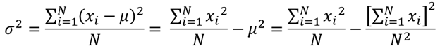
- The variance of X is equal to
the mean of the square of X minus the square of the mean of X. This equation should not be used for computations using floating point arithmetic because it suffers from catastrophic cancellation if the two components of the equation are similar in magnitude.
-
-
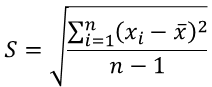
sample variance:
- one :
.png)
- other :
.png)
- The formula (Sn) will often undersstimate the actual population variance. And there's a formula, and actually proven more rigorously than I wil do it, that is considered to be a better. It's an unbiased estimate of the population variance.
- one :
-
-
Application scene:
- it measures how far a set of (random) numbers are spread out from their average value
标准差(standard deviation):
-
computational method:
- population standard deviation:
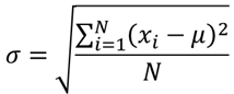
- sample standard deviaton:
- population standard deviation:
学员信息 学号:1901020015 学习内容:Exercise01-统计学知识 学习用时:236 学习笔记 <学习感悟>
variance 和 standard deviation还差一些,明天看完后开始学习 Tableau 。Tableau 的链接有中英文的,对我这种英文比较差的简直不能再友好,可以对照的看是一个幸福的事情
<学习笔记>
Exercise 01
英⽂文名称、计算方法、优点、缺点、应用场景
1、measuring the central tendency:
The arithmetic mean, median and mode can kind of be representative of a data sets or population central tendency. And they are all be forms of an 'average'.
In the other words, picking a number that is most representative of all the numbers.
And there no right answer, one of theses isn't a better answer for the average. They are just different ways of measuring the 'average'.
All three measures have the following property: If the random variable is subjected to the linear or affine transformation which replaces X by aX+b, so are the mean, median and mode.
均值(Arithmetic mean):
-
computational method:
- population mean:
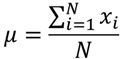
- sample mean:
- the sum of a collection of numbers divided by the count of numbers in the collection.
- population mean:
-
basic advantage:
- it is the most commonly used and readily understood measure of central tendency in a data set.
- The mean is the
only single numberfor which the residuals sum to zero - If the arithmetic mean of a population of numbers is desired, then the estimate of it that is unbiased is the arithmetic mean of a sample drawn from the population.
-
shortcoming:
- it is not a robust statistic, meaning that it is greatly influenced by outliers
-
Application scene:
- normally, used as a summary statistic, to indication the central tendency
- 通过样本平均数求整体平均数
中位数(Median):
以下为 Median of Finite Set Of Numbers, Median of Probability Distributions还没有读
Middle value separating the greater and lesser halves of a data set
-
computational method:
- Order these numbers from least to greatest
- If there is an odd number of numbers, the middle one is picked
- If there is an even number, the median is then usually defined to be the mean of the two middle values.
-
basic advantage:
- it is based on the middle data in a group, it is not necessary to even know the value of extreme results in order to calculate a median
- It is not skewed so much by a small proportion of extremely large or small values, and it is the
mostresistant statistic, so long as no more than half the data are contaminated, the median will not give an arbitrarily large or small result. - A median is only defined on ordered one-dimensional data, and is independent of any distance metric.
- A median can be worked out for ranked but not numerical classes
-
shortcoming:
- when data are uncontaminated by data from heavy-tailed distributions or from mixtures of distributions, it's not efficiency.
- While the data set isn't a linear order on the possible values, the median is not concept
-
Application scene:
- used as a summary statistic, to indication the central tendency for skewed distributions
- used as a measure of location when a distribution is skewed, when end-values are not known, or when one requires reduced importance to be attached to outliers
- used as a location parameter in descriptive statistics, like estimate the corresponding population values form a sample of data
-
Question: 关于效率这一点没搞明白
- More specifically, the median has a 64% efficiency compared to the minimum-variance mean (for large normal samples), which is to say the variance of the median will be ~50% greater than the variance of the mean—see asymptotic efficiency and references therein.
众数(mode):
The mode of a set of data values is the value that appears most often, it is the value that is most likely to be sampled.
The mode is not necessarily unique. Certain pathological distributions (for example, the Cantor distribution) have no defined mode at all
-
computational method:
- Most frequent value in a data set
-
basic advantage:
- The concept of mode also makes sense for "nominal data" (not numerical classes)
- Unlike median, the concept of mode makes sense for any random variable assuming values from a vector space, including the real numbers (like a distribution of points in the plane)
- Except for extremely small samples, the mode is insensitive to "outliers"
-
shortcoming:
- The mode is not necessarily unique to a given distribution, like discrete distribution, uniform distributions
中程数(mid-range):
The mid-range is the midpoint of the range(全距)
-
computational method:
-
- The mid-range or mid-extreme of a set of statistical data values is the arithmetic mean of the maximum and minimum values in a data set
-
-
computational method:
- It is the maximally efficient estimator for the center of a uniform distribution
- The midrange is a highly efficient estimator of μ, given a small sample of a sufficiently platykurtic distribution
-
shortcoming:
- It ignores all intermediate points, and lacks robustness, as outliers change it significantly. And having a breakdown point of 0. So, it lacks efficiency as an estimator for most distributions of interest and rarely used in practical statistical analysis
-
Application scene:
- Trimmed mid-ranges are also of interest as descriptive statistics or as L-estimators of central location or skewness: differences of mid-summaries, such as midhinge minus the median, give measures of skewness at different points in the tail
2、measuring the dispersion
these concept as above measuring the central tendency, but we lose a lot of information. we don't know whether all of the numbers in the data set are close to that number or maybe they're really far away from the mean. And thay's why we want to come up with measures of dispersion
方差(variance):
variance 的基本属性看了,深入属性还没有看
-
computational method:
-
population variance:
-
- The variance of X is equal to
the mean of the square of X minus the square of the mean of X. This equation should not be used for computations using floating point arithmetic because it suffers from catastrophic cancellation if the two components of the equation are similar in magnitude.
-
-
sample variance:
- one :
- other :
- The formula (Sn) will often undersstimate the actual population variance. And there's a formula, and actually proven more rigorously than I wil do it, that is considered to be a better. It's an unbiased estimate of the population variance.
- one :
-
-
Application scene:
- it measures how far a set of (random) numbers are spread out from their average value
标准差(standard deviation):
It is very important to note that the standard deviation of a population and the standard error of a statistic derived from that population are quite different but related
-
computational method:
- population standard deviation:
- sample standard deviaton:
- population standard deviation:
-
basic advantage:
- It is algebraically simpler, than the average absolute deviation.
- it is expressed in the same units as the data.
-
shortcoming:
- It is less robust, than the average absolute deviation.
-
Application scene:
- Used to quantify the amount of variation or dispersion of a set of data values
- The standard deviation is commonly used to measure confidence in statistical conclusions
全距(range):
-
computational method:
- The range of a set of data is the result of subtracting the smallest value from largest value
-
Application scene:
- Since it only depends on two of the observations, it is most useful in representing the dispersion of small data sets
-
**Question:**后面讲了很多“公式”,表示没有看懂。包括“For continuous IID random variables”、“For continuous non-IID random variables”、“For discrete IID random variables”
四分位数(quartile):
A quartile is a type of quantile. Have three quantile:
- Q1 (first quartile/lower quartile/25th percentile) : splits off the lowest 25% of data from the highest 75%
- Q2 (second quartile/median/50th percentile) : cuts data set in half
- Q3 (third quartile/upper quartile/75th percentile) : splits off the highest 25% of data from the lowest 75%
For discrete distributions, there is no universal agreement on selecting the quartile values.
-
computational method:
-
Method 1:
1.Use the median to divide the ordered data set into two halves.
- If there is an odd number of data points in the original ordered data set,
do not include the median(the central value in the ordered list) in either half. - If there is an even number of data points in the original ordered data set, split this data set exactly in half.
2.The lower quartile value is the median of the lower half of the data. The upper quartile value is the median of the upper half of the data.
- If there is an odd number of data points in the original ordered data set,
-
Method 2:
-
Use the median to divide the ordered data set into two halves.
-
If there are an odd number of data points in the original ordered data set,
include the median(the central value in the ordered list) in both halves. -
If there are an even number of data points in the original ordered data set, split this data set exactly in half.
-
-
The lower quartile value is the median of the lower half of the data. The upper quartile value is the median of the upper half of the data.
-
-
Method 3:
- If there are even numbers of data points, then Method 3 is the same as either method above
- If there are (4n+1) data points, then the lower quartile is 25% of the nth data value plus 75% of the (n+1)th data value; the upper quartile is 75% of the (3n+1)th data point plus 25% of the (3n+2)th data point.
- If there are (4n+3) data points, then the lower quartile is 75% of the (n+1)th data value
plus 25% of the (n+2)th data value; the upper quartile is25% of the (3n+2)th data pointplus 75% of the (3n+3)th data point.
-
-
Application scene:
-
quartile can computation interquartile range (IQR), and ICQ may be used to characterize the data when there may be extremities that skew the data. And fences are calculated using the following formula:
- Lower Fence = Q1 - 1.5(ICQ)
- Upper Fence = Q3 + 1.5(ICQ)
-
3、other
最大值和最小值(maximum/minimum):
Also called the largest observation and smallest observation, are the values of the greatest and least elements of a sample.
If the sample has outliers, they necessarily include the sample maximum or sample minimum, or both
-
computational method:
- Order these numbers from least to greatest
- The minimum and the maximum value are the first and last order sample
-
property: The sample maximum and minimum are the least robust statistics: they are maximally sensitive to outliers.
- basic advantage: if extreme values are real, and of real consequence, as in applications of extreme value theory( It seeks to assess, from a given ordered sample of a given random variable, the probability of events that are more extreme than any previously observed)
- shortcoming: if outliers have little or no impact on actual outcomes, then using non-robust statistics such as the sample extrema simply cloud the statistics
-
Application scene:
-
Showing the most extreme observations in the summary statistics (like five-number summary or seven-number summary and the associated box plot)
-
The sample maximum and minimum provide a prediction interval. A prediction interval is an estimate of an interval in which a future observation will fall, with a certain probability, given what has already been observed.
-
With clean data or in theoretical settings, maximum and minimum can sometimes prove very good estimators, particularly for platykurtic distributions, where for small data sets the mid-range is the most efficient estimator. But They are inefficient estimators of location for mesokurtic distributions. (The mid-range or mid-extreme of a set of statistical data values is the arithmetic mean of the maximum and minimum values in a data set)
-
For sampling without replacement from a uniform distribution with one or two unknown endpoints, maximum and minimum is an unbiased estimator derived from these will be UMVU estimator. (UMVU minimum-variance unbiased estimator)
-
The sample extrema can be used for a simple normality test, specifically of kurtosis: one computes the t-statistic of the sample maximum and minimum. If they are unusually large for the sample size, then the kurtosis of the sample distribution deviates significantly from that of the normal distribution.
-
Sample extrema play two main roles in extreme value theory:
- firstly, they give a lower bound on extreme events – events can be at least this extreme, and for this size sample;
- secondly, they can sometimes be used in estimators of probability of more extreme events.
-
学员信息 学号:1901020015 学习内容:Exercise01-统计学知识 学习用时:256 学习笔记 <学习感悟>
今天终于进入了Tableau的学习 Tableau Prep的视频是纯英的表示有点尴尬,果断看文档,基本是跟着文档做了一遍,文档中举到的例子和给到的对应数据源好像有一些出入,开始还很纠结很多东西对不上,后来就淡然了。只要明确每一步是做什么,会产生什么结果就好,不用太纠结细节。基本入门文档看完作业就可以完成,除了聚类那个步骤需要稍微多了解一下,不过不影响作业进度。 Tableau Desktop完成了第一个表格,明天继续把后面的图搞定。 整个过程走下来,目前的感觉是Tableau和Power BI有点像,不过Tableau Prep 的操作过程保留形成一个流程这一点超级赞。继续加油 [强壮]
学员信息 学号:1901020015 学习内容:Exercise01-Tableau/ Exercise02-可视化分析 学习用时:245 学习笔记 <学习感悟>
Tableau Destop 的资料先看了一遍视频,又看了一部分文本,感觉还是比较适合读文本。表示Tableau Destop的作业确实不难看一下轴合并就可以可以完成。截止今天Exercise01的内容算是全部完成了。
作业过了后拿到Exercise02的文档。先整体看可一遍,“可视化分析入门”这几个词吸引了我,点开看了看。里面三个核心概念:标记、粒度、故事,其实说白了就是选择什么图、展示要多细、再做个PPT。再往前看基本作业的内容也是围绕着这三个点展开的,那Exercise02以可视化分析为轴是没错了
之后,自己思考了一下,针对这两节做了一个串联。第一节的核心重点在于统计学知识(因为纯完成作业的话后面两个真的很好完成,特别是感觉Tableau Desktop的内容哪怕exercise01不看后面开始会学到)讲述了多个数据聚合离散程度的指标。目前来看第二节的重点应该在图的作用和选择,即用什么图表表示哪一类信息,或者别人用哪类图表在传递什么信息
另外,我好想改了这个issue的标题,表示好尴尬,不想重开一个issue写Exercise02
<学习笔记>
Exercise 02-可视化分析
可视化分析 - 是通过交互式可视化界面,从数据中获得知识和见解的过程
用 Tableau 可视化分析数据有两种方式:
- 直接开始探索
-
针对数据提出问题并尝试解答问题
相关概念:
- 标记(用什么图):我理解是可视化图表的样式,什么样的问题可以用什么图形表示是良好的分析起点
- 粒度(展示到多细):粒度是度量聚合的层次,由维度,以及所要求维度与标记间的交互方式设置
- 故事(写个PPT):分析的过程及思维的引导
学员信息 学号:1901020015 学习内容:Exercise01-Tableau/ Exercise02-可视化分析 学习用时:224 学习笔记
<学习感悟>
今天先把条形图、直方图、甘特图这一组看了一下,参照Exercise01的方式学习每个的优点、主要⽤用途及使⽤用场景,最后参照README的链接学习如何用Tableau制作。 另外今天自己总结提炼了一下,其实我昨天应该是解决了why的问题,就是这一节究竟要让我们学会什么,即可视化分析。现在在解决what和how的问题。继续加油
<学习笔记>
Exercise 02-可视化分析
统计图形
优点、主要⽤用途及使⽤用场景
条形图(Bar chart / bar graph):
-
Application: Shows comparisons among discrete categories.
-
Grouped bar charts and Stacked bar charts:
- In a grouped bar chart, for each categorical group there are two or more bars. These bars are color-coded to represent a particular grouping.
- The stacked bar chart stacks bars that represent different groups on top of each other. The height of the resulting bar shows the combined result of the groups.
- stacked bar charts are not suited to data sets where some groups have
negative values. In such cases, grouped bar chart are preferable.
直方图(Histogram):
It is an estimate of the probability distribution of a continuous variable (CORAL). And it yields a smoother probability density function, which will in general more accurately reflect distribution of the underlying variable.
The density estimate could be plotted as an alternative to the histogram. Histograms are nevertheless preferred in applications, when their statistical properties need to be modeled.
-
different with bar graph:
- a bar graph relates two variables, but a histogram relates only one.
- A histogram is used for continuous data, where the bins represent ranges of data, while a bar chart is a plot of categorical variables.
-
To construct a histogram:
-
Divide the entire range of values into a series of intervals.
-
Then count how many values fall into each interval.
-
Note that, the bins (intervals) must be adjacent, and are often (but are not required to be) of equal size.
- If the bins are of equal size, a rectangle is erected over the bin with height proportional to the
frequency—the number of cases in each bin. - If the bins are not of equal width, a rectangle is erected over the bin with height proportional to not the frequency but
frequency density—the number of cases per unit of the variable on the horizontal axis.
- If the bins are of equal size, a rectangle is erected over the bin with height proportional to the
-
-
Application:
- Histograms often for density estimation: estimating the probability density function of the underlying variable.
- The histogram is one of the seven basic tools of quality control.
-
Number of bins and width:
- Using wider bins where the density of the underlying data points is low reduces noise due to sampling randomness;
- Using narrower bins where the density is high (so the signal drowns the noise) gives greater precision to the density estimation.
- Thus varying the bin-width within a histogram can be beneficial. Nonetheless, equal-width bins are widely used.
- There are, however, various useful guidelines and rules of thumb
甘特图 (Gantt Chart):
A Gantt chart is a type of bar chart that illustrates a project schedule. Modern Gantt charts also show the dependency relationships between activities and current schedule status.
学员信息 学号:1901020015 学习内容:Exercise01-Tableau/ Exercise02-可视化分析 学习用时:244 学习笔记
<学习感悟>
今天先把甘特图看完了,折线图(趋势图)看了一部分,把这几个图的做法联系了几遍,开始有了一些感觉。
其实总使用上来说,就像在做PPT只不过有些东西换了一个地方,熟悉了就好。比较关键的有两个点,一个就是这个图用来做什么用要想清楚,另一个就是Tableau里面有一些不太一样的概念需要搞清楚,这也算是搞明白了为什么exercise02第一部分是相关概念的原因
今天有一个特别有感触的,就是“甘特图”,wiki上面讲述这主要用于项目流程管理,后来看Tableau文章的时候,是在用它显示一系列产品的平均交货时间。后来才突然反应过来,其实只要是和流程+时间序列相关的其实都可以用甘特图来表示。自己还是没有深入思考啊(它能用在哪里/还能用在哪里)
<学习笔记>
统计图形
甘特图 (Gantt Chart):
A Gantt chart is a type of bar chart that illustrates a project schedule, and are sometimes equated with bar charts. Modern Gantt charts also show the dependency relationships between activities and current schedule status.
Gantt charts are usually created initially using an early start time approach, where each task is scheduled to start immediately when its prerequisites are complete. This method maximizes the float time available for all tasks.
-
basic advantage:
- Gantt charts are easily interpreted without training
- 在甘特图中,每个单独的标记(通常是一个条形)显示一段持续时间。例如,您可以使用甘特图显示
一系列产品的平均交货时间【这样看来应该和流程+时间序列相关的都可以用甘特图】
-
Application:
- Gantt charts can be used to show current schedule status (using percent-complete shadings and a vertical "TODAY" line as shown here.)
-
Progress Gantt Chart:
- In a progress Gantt chart, tasks are shaded in proportion to the degree of their completio
- A vertical line is drawn at the time index when the progress Gantt chart is created, and this line can then be compared with shaded tasks. If everything is on schedule, all task portions left of the line will be shaded, and all task portions right of the line will not be shaded.
-
Linked Gantt Chart:
- Linked Gantt charts contain lines indicating the dependencies between tasks. However, linked Gantt charts quickly become cluttered in all but the simplest cases.
折线图(Line chart / line plot / line graph):
Charts often include an overlaid mathematical function depicting the best-fit trend of the scattered data. This layer is referred to as a best-fit layer and the graph containing this layer is often referred to as a line graph.
It is a type of chart which displays information as a series of data points called 'markers' connected by straight line segments.
-
basic advantage:
- the best-fit layer(Line chart) can reveal trends in the data.
- Measurements such as the gradient or the area under the curve can be made visually, leading to more conclusions or results from the data table
-
Application:
- Used to visualize a trend in data over intervals of time
Tableau 的相关定义
数据桶
- Tableau 中的任何离散字段都可以被认为是一组数据桶
- 当您利用度量创建数据桶时,您将创建一个新维度。这是因为您在
依据包含无限制连续值范围的字段创建包含一组有限、离散的可能值的字段。但是,一旦创建了维度,就可以将它转换为连续维度。这可能很有用,例如,如果要创建直方图。 - Tableau 用于计算最佳数据桶大小的公式为:Number of Bins = 3 + log2(n) * log(n)
- 向视图中添加分桶维度时,每个数据桶都充当一个大小相等的容器,用于对特定的值范围汇总数据
学员信息 学号:1901020015 学习内容:Exercise01-Tableau/ Exercise02-可视化分析 学习用时:253 学习笔记
<学习感悟>
今天先把饼图和散点图看完了气泡图看了一部分,看到气泡图的时候实在有点啃不动英文了,就转去Tableau做图去了。
- 饼图真的很逗比,是在科学界最不喜欢使用也是缺点最多的一个图形,但恰恰是变体最多的一个,不过也是因为对原饼图的改良感觉上也是好了很多。我就很喜欢Spie chart和Polar area diagram,但貌似tableau做不出来,后面再具体研究一下
- 散点图呢要特别控诉一下百度百科。开始不知道散点图的英文,所以百度百科了一下,百度百科里竟然说散布图 = 相关图。事实上有两个图形,一个是 ”Scatter plot-散点图“,一个是 ”correlogram-相关图/自相关图“,前者是用来观测两个变量的相关性的,后者是时间序列分析中用来检验样本自相关性的。**这两个不一样!
- 学习Tableau 做图还是比较 “玩的开” 的,喜欢把除了给到的链接外很多相关链接也读一读,感觉确实可以学到一些东西。具体性价比怎么样嘛,再容我研究把玩几天
<学习笔记>
饼图(pie chart / circle chart):
A pie chart is a circular statistical graphic, which is divided into slices to illustrate numerical proportion.
-
shortcoming:
- They cannot show more than a few values without separating the visual encoding from the data they represent
- It is difficult to compare different sections of a given pie chart, or to compare data across different pie charts.
Pie charts can be replaced in most cases by other plots such as the bar chart, box plot or dot plots. (in research performed at AT&T Bell Laboratories, it was shown that comparison by angle was less accurate than comparison by length. ) - Pie chart can't display other values such as averages or targets at the same time. It is more difficult for comparisons to be made between the size of items in a chart when area is used instead of length and when different items are shown as different shapes.
-
basic advantage:
- If the goal is to compare a given category (a slice of the pie) with the total (the whole pie) in a single chart and the multiple is close to 25 or 50 percent, then a pie chart can often be more effective than a bar graph.
-
Variants and similar charts:
-
Polar area diagram: The polar area diagram is similar to a usual pie chart, except sectors have equal angles and differ rather in how far each sector extends from the center of the circle. The polar area diagram is used to **
plot cyclic phenomena**【感觉和雷达图有点像,但雷达图好像不能做堆叠循环处理】 -
Ring chart, sunburst chart, and multilevel pie chart: It is used to
visualize hierarchical data, depicted by concentric circles. A segment of the inner circle bears a hierarchical relationship to those segments of the outer circle which lie within the angular sweep of the parent segment. - Spie chart: The base pie chart represents the first data set in the usual way, with different slice sizes. The second set is represented by the superimposed polar area chart, using the same angles as the base, and adjusting the radii to fit the data.【相当于用饼图的弧长和半径表现了两个维度】
- Square chart / Waffle chart: It is a form of pie charts that use squares instead of circles to represent percentages. The benefit to these is that it is easier to depict smaller percentages that would be hard to see on traditional pie charts.
-
Polar area diagram: The polar area diagram is similar to a usual pie chart, except sectors have equal angles and differ rather in how far each sector extends from the center of the circle. The polar area diagram is used to **
散布图/散点图(Scatter plot / scatter graph / scatter chart / scatter diagram):
百度百科里面有一个很坑的地方,就是说散布图 = 相关图。事实上有两个图形,一个是 ”Scatter plot-散点图“,一个是 ”correlogram-相关图/自相关图“,前者是用来观测两个变量的相关性的,后者是时间序列分析中用来检验样本自相关性的。这两个不一样!
It is a type of plot or mathematical diagram using Cartesian coordinates to display values for typically two variables for a set of data.
A scatter plot can be used either when one continuous variable that is under the control of the experimenter and the other depends on it or when both continuous variables are independent. And a scatter plot will illustrate only the degree of correlation (not causation) between two variables.
A scatter plot can suggest various kinds of correlations between variables with a certain confidence interval. Correlations may be positive (rising), negative (falling), or null (uncorrelated).
Scatter charts can be built in the form of bubble, marker, or/and line charts.
-
Application:
- Use to show correlations between variables.
- It is one of the seven basic tools of quality control.
气泡图(Bubble chart):
A bubble chart is a type of chart that displays three dimensions of data. Bubble charts can be considered a variation of the scatter plot, in which the data points are replaced with bubbles.
学员信息 学号:1901020015 学习内容:Exercise01-Tableau/ Exercise02-可视化分析 学习用时:67 学习笔记
<学习感悟>
今天先把气泡图看完了、热图看完了,点位图/填充地图看了一部分,相关的Tableau 的图表也一起做了做
- 气泡图有一个点自己曾经一直没有关注过,就是在第三个维度中数据是和面积相关的,所以数据间就会带来平方的差距而不是线性的。突然感觉自己无知无畏啊
- 填充地图这里英文是比较尬的,是“Choropleth map” ,之前自己搜了很多向“map”、“maps”、“shaded map”、“colored map”都没有找到,今天恰巧在热图这里发现了,万分开心。另外发现热图和自己之前理解有点不太一样,最开始是从矩阵数据着色发展起来的,之前基本把热力图和着色地图混为一谈
<学习笔记>
气泡图(Bubble chart):
A bubble chart is a type of chart that displays three dimensions of data. Bubble charts can be considered a variation of the scatter plot, in which the data points are replaced with bubbles.
-
shortcoming:
- it is area, rather than radius or diameter, that conveys the data.
- The area of a disk—unlike its diameter or circumference—is not proportional to its radius, but to the square of the radius.
- So if one chooses to scale the disks' radii to the third data values directly, then the apparent size differences among the disks will be non-linear (quadratic) and misleading. This scaling issue can lead to extreme misinterpretations, especially
where the range of the data has a large spread. - To get a properly weighted scale, one must scale each disk's radius to the square root of the corresponding data value v3. And it is important that bubble charts not only be scaled in this way, but also be clearly labeled to document that it is area, rather than radius or diameter, that conveys the data.
热图(Heat map):
A heat map is a graphical representation of data where the individual values contained in a matrix are represented as colors. "Heat map" is a newer term but shading matrices have existed for over a century.
学员信息 学号:1901020015 学习内容:Exercise01-Tableau/ Exercise02-可视化分析 学习用时:383 学习笔记
<学习感悟>
首先纠正一下昨天的错误,点位图/填充地图都是Thematic map的一种,而不是Choropleth map。这里花费了好多好多时间,Thematic map的种类好多种,也是蛮有意思的。另外把树形图看完了。相关的Tableau做了做
<学习笔记>
统计图形
地图/填充地图/着色地图(Thematic map)
A 'Thematic map' is a map that focuses on a specific theme or subject area. Thematic maps use the base data, such as coastlines, boundaries and places, only as points of reference for the phenomenon being mapped
General reference maps show where something is in space, thematic maps tell a story about that place
When designing a thematic map, cartographers must balance a number of factors in order to effectively represent the data. Besides spatial accuracy, and aesthetics, quirks of human visual perception and the presentation format must be taken into account.
-
Mapping methods:
-
-
Choropleth mapping shows statistical data aggregated over predefined regions, such as counties or states, by coloring or shading these regions.
-
This technique assumes a relatively even distribution of the measured phenomenon within each region.
-
Principles of color progression:
- Darker colors are perceived as being higher in magnitude
- Five to seven color categories are recommended
- Generally speaking, differences in hue are used to indicate qualitative differences, such as land use, while differences in saturation or lightness are used to indicate quantitative differences, such as population.
-
common error:
-
Choice of regions:【这里不是很理解,感觉上是不同粒度造成的统计差异,但为何dasymetric map可以折中这个问题没有明白】
- Where real-world patterns may not conform to the regions discussed, issues such as the ecological fallacy and the modifiable areal unit problem (MAUP) can lead to major misinterpretations, and other techniques are preferable. Similarly, the size and specificity of the displayed regions depend on the variable being represented. While the use of smaller and more specific regions can decrease the risk of ecological fallacy and MAUP, it can cause the map to appear to be more complicated. Although representing specific data in large regions can be misleading, it can make the map clearer and easier to interpret and remember. The choice of regions will ultimately depend on the map's intended audience and purpose.
- The dasymetric technique can be thought of as a compromise approach in many situations. (The dasymetric map)
-
Use of raw data values to represent magnitude rather than normalized values to produce a map of densities. A properly normalized map will show variables independent of the size of the polygons.【这一点一定要注意!】
-
-
-
Proportional symbol:
- The proportional symbol technique uses symbols of different heights, lengths, areas, or volumes to represent data associated with different areas or locations within the map.
- This type of map is useful for visualization when raw data cannot be dealt with as a ratio or proportion.
- Proportional symbol maps are effective because they allow the reader to understand large quantities of data in a fast and simple way.
- Note that, careful to use circles. The reason seam the pie chart
-
- A cartogram map is a map that purposely distorts geographic space based on values of a theme.
- Most commonly used in everyday life are distance cartograms. Distance cartograms show real-world distances that are distorted to reflect some sort of attribute.
- Another type of cartogram is an area cartogram. These are created by scaling (or sizing) enumeration units as a function of the values of an attribute associated with the enumeration units. There are two different forms of an area cartogram: contiguous and noncontiguous.
- (说白了就是一个将长度按数据比例缩放,另一个将面积按数据比例缩放,一个是line,一个是square)
-
- Isarithmic maps, also known as contour maps or isoline maps depict smooth continuous phenomena
- An Isarithmic map is a planimetric graphic representation of a 3-D surface.
-
-
A dot distribution map might be used to locate each occurrence of a phenomenon
-
Where appropriate, the dot distribution technique may also be used in combination the proportional symbol technique
-
shortcoming:【对于这里不是很理解,点位图应该是根据实际的位置坐标确定的啊,为什么会存在位置不准确问题呢,而且点位图的点不应该是相同的吗又为何会存在主观的大小和间距问题呢?】
- One such disadvantage is that the actual dot placement may be random. That is, there may be no actual phenomenon where the dots are located.
- The subjective nature of the dot size and spacing could give the map a biased view. Inappropriately sized or spaced dots can skew or distort the message a map attempts to communicate. If the dots are too numerous, it may be difficult for the reader to count the dots.
-
-
Flow:
- Flow maps are maps that use lines or arrows to portray movement between two or more destinations.
- These lines or arrows can also represent quantities of things being transferred between locations. This can be done via use of proportional symbols.
-
- A dasymetric map is an alternative to a choropleth map.
- As with a choropleth map, data are collected by enumeration units. But instead of mapping the data so that the region appears uniform, ancillary information(like forest, water, grassland, urbanization) is used to model internal distribution of the phenomenon.
-
树形图
In probability theory, a tree diagram may be used to represent a probability space.
Tree diagrams may represent a series of independent events or conditional probabilities. Each node on the diagram represents an event and is associated with the probability of that event. The root node represents the certain event and therefore has probability 1. Each set of sibling nodes represents an exclusive and exhaustive partition of the parent event.
Tableau 的相关内容
散点图
- 在 Tableau 中,可以通过在“列”功能区和“行”功能区上分别放置至少一个度量来创建散点图。如果这些功能区同时包含维度和度量,则 Tableau 会将度量设置为最内层字段,这意味着度量始终位于您同样放置在这些功能区上的任何维度的右侧
学员信息 学号:1901020015 学习内容:Exercise01-Tableau/ Exercise02-可视化分析 学习用时:245 学习笔记
<学习感悟>
今天把箱型图、标靶图看完了,表示突出显示表确实没有找到相关信息。第一部分中Tableau要求及基础知识也看了一遍,关于标记的内容之前已经看完了,剩下的内容中我觉得寻址和分区哪里是需要着重理解以下的。特别是在使用“计算依据”的时候分区的排序就很重要,不过这里有一个简单的理解方法:你把它想成for循环,前面的就是外面的for循环,后面的就是里面的for循环就好了。 内容看完,明天完成仪表盘和故事,走起~
对了还有一个内容需要明天看一下:误导性图表。这个是自己开发出来的,我理解这一节最重要的是明确在什么情况下使用什么图,那对于不同图可能造成的误导偏差需要做进一步的了解。目前印象比较深刻的,过程中读到的有两种,第一种是圆形由于是square所以会造成视觉误差(容易产生在饼图、点位图这些圆形标记的位置)另一种就是填充地图,数据采用的是没有处理过的原始数据而不是与面积无关的密度数据,会造成数据反差
<学习笔记>
统计图形
优点、主要⽤用途及使⽤用场景
箱型图(Box plot)
Box plots are non-parametric: they display variation in samples of a statistical population without making any assumptions of the underlying statistical distribution
In addition to the points themselves, they allow one to visually estimate various L-estimators, notably the interquartile range, midhinge, range, mid-range, and trimean.
-
The end of whiskers:
-
the minimum and maximum of all of the data
-
the lowest datum still within 1.5 IQR of the lower quartile, and the highest datum still within 1.5 IQR of the upper quartile (often called the Tukey boxplot)
- The interquartile range (IQR) is a measure of statistical dispersion, being equal to the difference between 75th and 25th percentiles, or between upper and lower quartiles IQR = Q3 − Q1.
-
one standard deviation above and below the mean of the data
-
the 9th percentile and the 91st percentile
-
the 2nd percentile and the 98th percentile.
-
-
advantage:
- They take up less space and are therefore particularly useful for comparing distributions between several groups or sets of data (Box plot / Histogram / Kernel density estimate)
标靶图/子弹图(Bullet graph)
The bullet graph serves as a replacement for dashboard gauges and meters.
The bullet graph features a single, primary measure, compares that measure to one or more other measures to enrich its meaning, and displays it in the context of qualitative ranges of performance, such as poor, satisfactory, and good.
Tableau 的相关内容
代表性标记
-
文本标记:
- 如果“行”和“列”功能区上的内部字段
都是维度,则会自动选择“文本”标记类型 - 此类型适用于显示与一个或多个维度成员关联的数字。此类视图通常称为文本表、交叉表或数据透视表
- 如果“行”和“列”功能区上的内部字段
-
形状标记:
- 如果“行”和“列”功能区上的内部字段
都是度量,则会选择“形状”标记类型。 - 此类型适用于 清晰呈现各个数据点以及与这些数据点关联的类别
- 形状属性:如果字段是 维度,则为每个成员分配一个唯一形状。如果字段是 度量,则将该度量自动分级到不同的存储桶中,并为每个存储桶分配一个唯一形状
- 如果“行”和“列”功能区上的内部字段
-
条形标记:
- 如果“行”和“列”功能区上的内部字段是
维度和度量,则会选择“条形”标记类型。 - 此类型适用于比较各种类别间的度量,或用于将数据分成堆叠条
- 如果“行”和“列”功能区上的内部字段是
-
线形标记:
-
如果“行”和“列”功能区上的内部字段是
日期字段和度量,则会选择“线”标记类型 -
此类型适用于查看数据随时间的变化趋势,数据排列顺序,或者是否有必要进行插补
-
路径属性中分为线性、阶梯、跳跃:
- 线性;为在一段时间内保持不变并且变化或增量显著的数值数据*(例如帐户余额、库存水平或利率)*
- 阶梯:非常适合用于强调变化的量级
- 跳跃:可帮助强调数据点之间变化的持续时间
-
-
区域标记:
- 适用于视图标记堆叠而不重叠的情况(我理解是线的延伸,面积图)
-
堆叠标记:(这个标记需要在“分析”中寻找)
- 当数据视图中包含数字轴时适合使用堆叠标记。也就是说,至少已将一个度量放在“行”或“列”功能区上。
- 堆叠的标记沿轴合并绘制。未堆叠的标记沿轴单独绘制。也就是说,它们是重叠的。
- 通过选择**“分析”>“堆叠标记”**菜单项,您可以在任何给定视图中控制标记是堆叠还是重叠
- 对条堆积 —> 堆积条形图,对线堆积 —> 面积图
-
多边形标记:
- 多边形由点和区域外围的线连接而成
- 多边形标记不常使用,通常只适合具有特殊结构的数据源
-
密度标记:
- 适用于来呈现包含许多重叠标记的密度数据中的模式或趋势
表计算
对于任何 Tableau 可视化项,都有一个由视图中的维度确定的虚拟表。虚拟表由“详细信息级别”内的维度来决定
-
分区字段:
- 用于定义计算分组方式(执行表计算所针对的数据范围)的维度称为分区字段
- 分区字段会将视图拆分成多个子视图(或子表),然后将表计算应用于每个此类分区内的标记
- 【分区维度的顺序,我立即为多个不同的for循环的组合,最上面的是最外层的for循环最下面的是最里层的for循环】
-
寻址字段:
- 执行表计算所针对的其余维度称为寻址字段,可确定计算方向
- 计算移动的方向由寻址字段来决定(例如,在计算汇总或计算值之间的差值过程中)
- 当您使用“计算依据”选项添加表计算时,Tableau 会根据您的选择自动将某些维度确定为寻址维度,将其他维度确定为分区维度
-
移动计算:
- 对于视图中的每个标记,“移动计算”表计算会对当前值之前和/或之后指定数目的值执行聚合*(总计值、平均值、最小值或最大值)*来确定视图中的标记值。
- 移动计算通常用于平滑短期数据波动,这样可以查看长期趋势。
学员信息 学号:1901020015 学习内容:Exercise01-Tableau/ Exercise02-可视化分析 学习用时:365 学习笔记
<学习感悟>
开始花了很多时间去倒腾究竟要分析什么,最后确定了做一个销售分析好了基本思路如下: 1、看销售额基本趋势,并拆解为活跃客户数、销售数量、销售单价三个维度,得出结论:连续四年销售额持续增长,增幅加快。其原因主要是客户购买数量提升 2、以第一个的结果作为后续的问题,提出两个问题:1)单客户购买数量提升是频率提高了还是单客户购买的品类多了;2)客户增长降低是什么原因 3、一个问题一个问题解答,先解答客户的问题,主要对活跃客户做留存分析。拆解为三个方向,不同类型客户降幅增幅情况、活跃客户进入年份分布、各区域差异。最后得出结论:用户数量的提升当前主要依靠老客户激活,在销售单价不变的情况下会快速到达销售增量瓶颈。同时不同类型不同区域的新增数均基本同比例下滑。需要结合市场容量、获客渠道、人均效能做进一步判断,看是需要进一步提升单客户购买力还是拉升客户数量 4、继续解答另一个问题,即购买数量提升的原因。也是从三个方面解答,单客户年购买数量、单客户年购买频率、购买品类数。最后得出结论:可以发现客户在购买数量和频次上均有所上升,办公用品的购买数数量尤为明显,客户在三个品类的购买频率中上升幅度基本同步。同时购买的产品类别数基本没变
这个过程中遇到的最大的问题就是需要写创建好几个计算字段基本都会用到“详细级别表达式”,好的一点就是FIXED都可以搞定,剩下两个详细级别表达式也还没来的级看
<学习笔记> 今天放完整的好了,后续如果会做优化就直接对这篇修改好了
Exercise 02-可视化分析
可视化分析 - 是通过交互式可视化界面,从数据中获得知识和见解的过程
用 Tableau 可视化分析数据有两种方式:
- 直接开始探索
-
针对数据提出问题并尝试解答问题
相关概念:
- 标记(用什么图):我理解是可视化图表的样式,什么样的问题可以用什么图形表示是良好的分析起点
- 粒度(展示到多细):粒度是度量聚合的层次,由维度,以及所要求维度与标记间的交互方式设置
- 故事(写个PPT):分析的过程及思维的引导
统计图形
优点、主要⽤用途及使⽤用场景
条形图(Bar chart / bar graph)
-
Application: Shows comparisons among discrete categories.
-
Grouped bar charts and Stacked bar charts:
- In a grouped bar chart, for each categorical group there are two or more bars. These bars are color-coded to represent a particular grouping.
- The stacked bar chart stacks bars that represent different groups on top of each other. The height of the resulting bar shows the combined result of the groups.
- stacked bar charts are not suited to data sets where some groups have
negative values. In such cases, grouped bar chart are preferable.
直方图(Histogram)
It is an estimate of the probability distribution of a continuous variable (CORAL). And it yields a smoother probability density function, which will in general more accurately reflect distribution of the underlying variable.
The density estimate could be plotted as an alternative to the histogram. Histograms are nevertheless preferred in applications, when their statistical properties need to be modeled.
-
different with bar graph:
- a bar graph relates two variables, but a histogram relates only one.
- A histogram is used for continuous data, where the bins represent ranges of data, while a bar chart is a plot of categorical variables.
-
To construct a histogram:
-
Divide the entire range of values into a series of intervals.
-
Then count how many values fall into each interval.
-
Note that, the bins (intervals) must be adjacent, and are often (but are not required to be) of equal size.
- If the bins are of equal size, a rectangle is erected over the bin with height proportional to the
frequency—the number of cases in each bin. - If the bins are not of equal width, a rectangle is erected over the bin with height proportional to not the frequency but
frequency density—the number of cases per unit of the variable on the horizontal axis.
- If the bins are of equal size, a rectangle is erected over the bin with height proportional to the
-
-
Application:
- Histograms often for density estimation: estimating the probability density function of the underlying variable.
- The histogram is one of the seven basic tools of quality control.
-
Number of bins and width:
- Using wider bins where the density of the underlying data points is low reduces noise due to sampling randomness;
- Using narrower bins where the density is high (so the signal drowns the noise) gives greater precision to the density estimation.
- Thus varying the bin-width within a histogram can be beneficial. Nonetheless, equal-width bins are widely used.
- There are, however, various useful guidelines and rules of thumb
箱型图(Box plot)
Box plots are non-parametric: they display variation in samples of a statistical population without making any assumptions of the underlying statistical distribution
In addition to the points themselves, they allow one to visually estimate various L-estimators, notably the interquartile range, midhinge, range, mid-range, and trimean.
-
The end of whiskers:
-
the minimum and maximum of all of the data
-
the lowest datum still within 1.5 IQR of the lower quartile, and the highest datum still within 1.5 IQR of the upper quartile (often called the Tukey boxplot)
- The interquartile range (IQR) is a measure of statistical dispersion, being equal to the difference between 75th and 25th percentiles, or between upper and lower quartiles IQR = Q3 − Q1.
-
one standard deviation above and below the mean of the data
-
the 9th percentile and the 91st percentile
-
the 2nd percentile and the 98th percentile.
-
-
advantage:
- They take up less space and are therefore particularly useful for comparing distributions between several groups or sets of data (Box plot / Histogram / Kernel density estimate)
甘特图 (Gantt Chart)
A Gantt chart is a type of bar chart that illustrates a project schedule, and are sometimes equated with bar charts. Modern Gantt charts also show the dependency relationships between activities and current schedule status.
Gantt charts are usually created initially using an early start time approach, where each task is scheduled to start immediately when its prerequisites are complete. This method maximizes the float time available for all tasks.
-
basic advantage:
- Gantt charts are easily interpreted without training
- 在甘特图中,每个单独的标记(通常是一个条形)显示一段持续时间。例如,您可以使用甘特图显示
一系列产品的平均交货时间【这样看来应该和流程+时间序列相关的都可以用甘特图】
-
Application:
- Gantt charts can be used to show current schedule status (using percent-complete shadings and a vertical "TODAY" line as shown here.)
-
Progress Gantt Chart:
- In a progress Gantt chart, tasks are shaded in proportion to the degree of their completio
- A vertical line is drawn at the time index when the progress Gantt chart is created, and this line can then be compared with shaded tasks. If everything is on schedule, all task portions left of the line will be shaded, and all task portions right of the line will not be shaded.
-
Linked Gantt Chart:
- Linked Gantt charts contain lines indicating the dependencies between tasks. However, linked Gantt charts quickly become cluttered in all but the simplest cases.
标靶图/子弹图(Bullet graph)
The bullet graph serves as a replacement for dashboard gauges and meters.
The bullet graph features a single, primary measure, compares that measure to one or more other measures to enrich its meaning, and displays it in the context of qualitative ranges of performance, such as poor, satisfactory, and good.
折线图(Line chart / line plot / line graph)
Charts often include an overlaid mathematical function depicting the best-fit trend of the scattered data. This layer is referred to as a best-fit layer and the graph containing this layer is often referred to as a line graph.
It is a type of chart which displays information as a series of data points called 'markers' connected by straight line segments.
-
basic advantage:
- the best-fit layer(Line chart) can reveal trends in the data.
- Measurements such as the gradient or the area under the curve can be made visually, leading to more conclusions or results from the data table
-
shortcoming:
- Line charts should be used for numerical data only, and not categorical.
-
Application:
- Used to visualize a trend in data over intervals of time
饼图(pie chart / circle chart)
A pie chart is a circular statistical graphic, which is divided into slices to illustrate numerical proportion.
-
shortcoming:
- They cannot show more than a few values without separating the visual encoding from the data they represent
- It is difficult to compare different sections of a given pie chart, or to compare data across different pie charts.
Pie charts can be replaced in most cases by other plots such as the bar chart, box plot or dot plots. (in research performed at AT&T Bell Laboratories, it was shown that comparison by angle was less accurate than comparison by length. ) - Pie chart can't display other values such as averages or targets at the same time. It is more difficult for comparisons to be made between the size of items in a chart when area is used instead of length and when different items are shown as different shapes.
-
basic advantage:
- If the goal is to compare a given category (a slice of the pie) with the total (the whole pie) in a single chart and the multiple is close to 25 or 50 percent, then a pie chart can often be more effective than a bar graph.
-
Variants and similar charts:
-
Polar area diagram: The polar area diagram is similar to a usual pie chart, except sectors have equal angles and differ rather in how far each sector extends from the center of the circle. The polar area diagram is used to **
plot cyclic phenomena**【感觉和雷达图有点像,但雷达图好像不能做堆叠循环处理】 -
Ring chart, sunburst chart, and multilevel pie chart: It is used to
visualize hierarchical data, depicted by concentric circles. A segment of the inner circle bears a hierarchical relationship to those segments of the outer circle which lie within the angular sweep of the parent segment. - Spie chart: The base pie chart represents the first data set in the usual way, with different slice sizes. The second set is represented by the superimposed polar area chart, using the same angles as the base, and adjusting the radii to fit the data.【相当于用饼图的弧长和半径表现了两个维度】
- Square chart / Waffle chart: It is a form of pie charts that use squares instead of circles to represent percentages. The benefit to these is that it is easier to depict smaller percentages that would be hard to see on traditional pie charts.
-
Polar area diagram: The polar area diagram is similar to a usual pie chart, except sectors have equal angles and differ rather in how far each sector extends from the center of the circle. The polar area diagram is used to **
散布图/散点图(Scatter plot / scatter graph / scatter chart / scatter diagram)
百度百科里面有一个很坑的地方,就是说散布图 = 相关图。事实上有两个图形,一个是 ”Scatter plot-散点图“,一个是 ”correlogram-相关图/自相关图“,前者是用来观测两个变量的相关性的,后者是时间序列分析中用来检验样本自相关性的。这两个不一样!
It is a type of plot or mathematical diagram using Cartesian coordinates to display values for typically two variables for a set of data.
A scatter plot can be used either when one continuous variable that is under the control of the experimenter and the other depends on it or when both continuous variables are independent. And a scatter plot will illustrate only the degree of correlation (not causation) between two variables.
A scatter plot can suggest various kinds of correlations between variables with a certain confidence interval. Correlations may be positive (rising), negative (falling), or null (uncorrelated).
Scatter charts can be built in the form of bubble, marker, or/and line charts.
-
Application:
- Use to show correlations between variables.
- It is one of the seven basic tools of quality control.
气泡图(Bubble chart)
A bubble chart is a type of chart that displays three dimensions of data. Bubble charts can be considered a variation of the scatter plot, in which the data points are replaced with bubbles.
-
shortcoming:
-
it is area, rather than radius or diameter, that conveys the data.
- The area of a disk—unlike its diameter or circumference—is not proportional to its radius, but to the square of the radius.
- So if one chooses to scale the disks' radii to the third data values directly, then the apparent size differences among the disks will be non-linear (quadratic) and misleading. This scaling issue can lead to extreme misinterpretations, especially
where the range of the data has a large spread. - To get a properly weighted scale, one must scale each disk's radius to the square root of the corresponding data value v3. And it is important that bubble charts not only be scaled in this way, but also be clearly labeled to document that it is area, rather than radius or diameter, that conveys the data.
-
热图(Heat map)
A heat map is a graphical representation of data where the individual values contained in a matrix are represented as colors. "Heat map" is a newer term but shading matrices have existed for over a century.
地图/填充地图/着色地图(Thematic map)
A 'Thematic map' is a map that focuses on a specific theme or subject area. Thematic maps use the base data, such as coastlines, boundaries and places, only as points of reference for the phenomenon being mapped
General reference maps show where something is in space, thematic maps tell a story about that place
When designing a thematic map, cartographers must balance a number of factors in order to effectively represent the data. Besides spatial accuracy, and aesthetics, quirks of human visual perception and the presentation format must be taken into account.
-
Mapping methods:
-
-
Choropleth mapping shows statistical data aggregated over predefined regions, such as counties or states, by coloring or shading these regions.
-
This technique assumes a relatively even distribution of the measured phenomenon within each region.
-
Principles of color progression:
- Darker colors are perceived as being higher in magnitude
- Five to seven color categories are recommended
- Generally speaking, differences in hue are used to indicate qualitative differences, such as land use, while differences in saturation or lightness are used to indicate quantitative differences, such as population.
-
common error:
-
Choice of regions:【这里不是很理解,感觉上是不同粒度造成的统计差异,但为何dasymetric map可以折中这个问题没有明白】
- Where real-world patterns may not conform to the regions discussed, issues such as the ecological fallacy and the modifiable areal unit problem (MAUP) can lead to major misinterpretations, and other techniques are preferable. Similarly, the size and specificity of the displayed regions depend on the variable being represented. While the use of smaller and more specific regions can decrease the risk of ecological fallacy and MAUP, it can cause the map to appear to be more complicated. Although representing specific data in large regions can be misleading, it can make the map clearer and easier to interpret and remember. The choice of regions will ultimately depend on the map's intended audience and purpose.
- The dasymetric technique can be thought of as a compromise approach in many situations. (The dasymetric map)
-
Use of raw data values to represent magnitude rather than normalized values to produce a map of densities. A properly normalized map will show variables independent of the size of the polygons.【这一点一定要注意!】
-
-
-
Proportional symbol:
- The proportional symbol technique uses symbols of different heights, lengths, areas, or volumes to represent data associated with different areas or locations within the map.
- This type of map is useful for visualization when raw data cannot be dealt with as a ratio or proportion.
- Proportional symbol maps are effective because they allow the reader to understand large quantities of data in a fast and simple way.
- Note that, careful to use circles. The reason seam the pie chart
-
- A cartogram map is a map that purposely distorts geographic space based on values of a theme.
- Most commonly used in everyday life are distance cartograms. Distance cartograms show real-world distances that are distorted to reflect some sort of attribute.
- Another type of cartogram is an area cartogram. These are created by scaling (or sizing) enumeration units as a function of the values of an attribute associated with the enumeration units. There are two different forms of an area cartogram: contiguous and noncontiguous.
- (说白了就是一个将长度按数据比例缩放,另一个将面积按数据比例缩放,一个是line,一个是square)
-
- Isarithmic maps, also known as contour maps or isoline maps depict smooth continuous phenomena
- An Isarithmic map is a planimetric graphic representation of a 3-D surface.
-
-
A dot distribution map might be used to locate each occurrence of a phenomenon
-
Where appropriate, the dot distribution technique may also be used in combination the proportional symbol technique
-
shortcoming:【对于这里不是很理解,点位图应该是根据实际的位置坐标确定的啊,为什么会存在位置不准确问题呢,而且点位图的点不应该是相同的吗又为何会存在主观的大小和间距问题呢?】
- One such disadvantage is that the actual dot placement may be random. That is, there may be no actual phenomenon where the dots are located.
- The subjective nature of the dot size and spacing could give the map a biased view. Inappropriately sized or spaced dots can skew or distort the message a map attempts to communicate. If the dots are too numerous, it may be difficult for the reader to count the dots.
-
-
Flow:
- Flow maps are maps that use lines or arrows to portray movement between two or more destinations.
- These lines or arrows can also represent quantities of things being transferred between locations. This can be done via use of proportional symbols.
-
- A dasymetric map is an alternative to a choropleth map.
- As with a choropleth map, data are collected by enumeration units. But instead of mapping the data so that the region appears uniform, ancillary information(like forest, water, grassland, urbanization) is used to model internal distribution of the phenomenon.
-
树形图(Tree Diagram)
In probability theory, a tree diagram may be used to represent a probability space.
Tree diagrams may represent a series of independent events or conditional probabilities. Each node on the diagram represents an event and is associated with the probability of that event. The root node represents the certain event and therefore has probability 1. Each set of sibling nodes represents an exclusive and exhaustive partition of the parent event.
突出显示图
Tableau 的相关内容
数据桶
- Tableau 中的任何离散字段都可以被认为是一组数据桶
- 当您利用度量创建数据桶时,您将创建一个新维度。这是因为您在
依据包含无限制连续值范围的字段创建包含一组有限、离散的可能值的字段。但是,一旦创建了维度,就可以将它转换为连续维度。这可能很有用,例如,如果要创建直方图。 - Tableau 用于计算最佳数据桶大小的公式为:Number of Bins = 3 + log2(n) * log(n)
- 向视图中添加分桶维度时,每个数据桶都充当一个大小相等的容器,用于对特定的值范围汇总数据
散点图
- 在 Tableau 中,可以通过在“列”功能区和“行”功能区上分别放置至少一个度量来创建散点图。如果这些功能区同时包含维度和度量,则 Tableau 会将度量设置为最内层字段,这意味着度量始终位于您同样放置在这些功能区上的任何维度的右侧
代表性标记
-
文本标记:
- 如果“行”和“列”功能区上的内部字段
都是维度,则会自动选择“文本”标记类型 - 此类型适用于显示与一个或多个维度成员关联的数字。此类视图通常称为文本表、交叉表或数据透视表
- 如果“行”和“列”功能区上的内部字段
-
形状标记:
- 如果“行”和“列”功能区上的内部字段
都是度量,则会选择“形状”标记类型。 - 此类型适用于 清晰呈现各个数据点以及与这些数据点关联的类别
- 形状属性:如果字段是 维度,则为每个成员分配一个唯一形状。如果字段是 度量,则将该度量自动分级到不同的存储桶中,并为每个存储桶分配一个唯一形状
- 如果“行”和“列”功能区上的内部字段
-
条形标记:
- 如果“行”和“列”功能区上的内部字段是
维度和度量,则会选择“条形”标记类型。 - 此类型适用于比较各种类别间的度量,或用于将数据分成堆叠条
- 如果“行”和“列”功能区上的内部字段是
-
线形标记:
-
如果“行”和“列”功能区上的内部字段是
日期字段和度量,则会选择“线”标记类型 -
此类型适用于查看数据随时间的变化趋势,数据排列顺序,或者是否有必要进行插补
-
路径属性中分为线性、阶梯、跳跃:
- 线性;为在一段时间内保持不变并且变化或增量显著的数值数据*(例如帐户余额、库存水平或利率)*
- 阶梯:非常适合用于强调变化的量级
- 跳跃:可帮助强调数据点之间变化的持续时间
-
-
区域标记:
- 适用于视图标记堆叠而不重叠的情况(我理解是线的延伸,面积图)
-
堆叠标记:(这个标记需要在“分析”中寻找)
- 当数据视图中包含数字轴时适合使用堆叠标记。也就是说,至少已将一个度量放在“行”或“列”功能区上。
- 堆叠的标记沿轴合并绘制。未堆叠的标记沿轴单独绘制。也就是说,它们是重叠的。
- 通过选择**“分析”>“堆叠标记”**菜单项,您可以在任何给定视图中控制标记是堆叠还是重叠
- 对条堆积 —> 堆积条形图,对线堆积 —> 面积图
-
多边形标记:
- 多边形由点和区域外围的线连接而成
- 多边形标记不常使用,通常只适合具有特殊结构的数据源
-
密度标记:
- 适用于来呈现包含许多重叠标记的密度数据中的模式或趋势
表计算
对于任何 Tableau 可视化项,都有一个由视图中的维度确定的虚拟表。虚拟表由“详细信息级别”内的维度来决定
-
分区字段:
- 用于定义计算分组方式(执行表计算所针对的数据范围)的维度称为分区字段
- 分区字段会将视图拆分成多个子视图(或子表),然后将表计算应用于每个此类分区内的标记
- 【分区维度的顺序,我立即为多个不同的for循环的组合,最上面的是最外层的for循环最下面的是最里层的for循环】
-
寻址字段:
- 执行表计算所针对的其余维度称为寻址字段,可确定计算方向
- 计算移动的方向由寻址字段来决定(例如,在计算汇总或计算值之间的差值过程中)
- 当您使用“计算依据”选项添加表计算时,Tableau 会根据您的选择自动将某些维度确定为寻址维度,将其他维度确定为分区维度
-
移动计算:
- 对于视图中的每个标记,“移动计算”表计算会对当前值之前和/或之后指定数目的值执行聚合*(总计值、平均值、最小值或最大值)*来确定视图中的标记值。
- 移动计算通常用于平滑短期数据波动,这样可以查看长期趋势。
详细级别表达式
-
行级别表达式:
- 例如:
[Sales] / [Profit] - 在基础表中的每一行计算引用非聚合数据源列的表达式,此表达式在每行进行计算,并生成一个包含结果的新列
- 例如:
-
视图级别表达式:
- 例如:
SUM(Sales) / SUM(Profit) - 引用聚合数据源列的表达式将在视图中的维度所定义的维度处进行计算。如果将此计算拖到功能区,则 Tableau 会将其放在 AGG 函数内,表示它是聚合计算,并且无法进一步聚合
- 例如:
-
表范围详细级别表达式:
- 例如:
{MIN([Order Date])}={FIXED : MIN([Order Date])} - 可以在不使用任何定界关键字的情况下在表级别定义详细级别表达式,这相当于没有维度声明的 FIXED 详细级别表达式:
- 例如:
-
FIXED 详细级别表达式
- 例如:
{FIXED : MIN([Order Date])} - FIXED 详细级别表达式使用指定的维度计算值,而不引用视图中的维度。FIXED 详细级别表达式可能会生成度量或维度,具体情况视聚合表达式中的基础字段而定
- FIXED 详细级别表达式的详细级别可能比视图更精细、更粗略或与之相同。是否需要对 FIXED 详细级别的结果进行聚合取决于视图中有什么维度
- 例如:
-
INCLUDE 详细级别表达式
- INCLUDE 详细级别表达式始终是度量
- INCLUDE 详细级别将与视图相同或比视图更精细。因此,值将从不会重复
-
EXCLUDE 详细级别表达式
- EXCLUDE 详细级别表达式始终是度量
- EXCLUDE 详细级别表达式始终会导致视图中出现重复值。将包括 EXCLUDE 详细级别表达式的计算放在功能区上时,Tableau 默认情况下将进行 ATTR 聚合(而不是 SUM 或 AVG)以指明表达式实际上并未在聚合,并且更改聚合将不会影响视图
-
视图的详细级别表达式:
- 视图的详细级别确定视图中标记的数量,向视图中添加详细级别表达式时,Tableau 必须协调两个详细级别:视图中的详细级别以及表达式中的详细级别
学员信息 学号:1901020015 学习内容:Exercise02-可视化分析 学习用时:200 学习笔记
<学习感悟>
今天发生了一件超级尴尬的事情——作业竟然被退回来了。自己研究了一下,发现自己没有好好看作业,把一个简单的问题做复杂了,却没有完成作业。作业明明只是要做图表讲图表,自己却实实在在的做了一场分析……
想着既然退回来了,打打基础好了,边完成作业边把之前看的内容再学习了一遍。最后以作业故事的开篇结束吧
学员信息 学号:1901020015 学习内容:Exercise03-地图数据分析 学习用时:257 学习笔记
<学习感悟>
今天把Tableau 中的地图和地理数据分析完整看完,里面的图表都练习了一遍,也把exercise03的作业完成了。其实只要把Tableau 中的地图和地理数据分析完整看完,作业完全没有问题
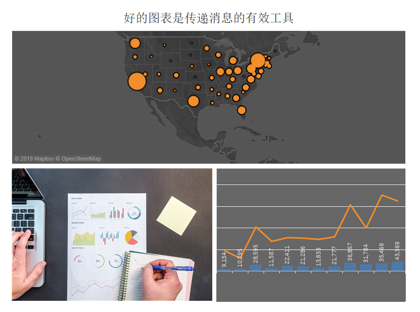
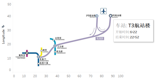
比较容易出问题的是作业2,今天的作业2开始没有特别理解做成了下面这个样子
 但是总觉得教练给的图片怎么能没用上呢,于是就和教练沟通了一下,所以下面这句话是最重要的:
在工作表中绘制背景地图:北北京机场线 意思是 以图片background为背景图片而不使用地图,在这个基础上完成后续的内容
最后在领悟了真谛后我做成了下面这个样子
但是总觉得教练给的图片怎么能没用上呢,于是就和教练沟通了一下,所以下面这句话是最重要的:
在工作表中绘制背景地图:北北京机场线 意思是 以图片background为背景图片而不使用地图,在这个基础上完成后续的内容
最后在领悟了真谛后我做成了下面这个样子
大功告成后开始了作业4。作业4先看了一遍,高级图表给的是视频,跟着做就行。预测的需要把文本只是看一下。但后来我发现高级图表也有文本知识,所以准备exercise04这样完成: 1、按照视频把作业做了 2、按照把文本的高级图表知识看完 3、把预测作业完成
<学习笔记>
Exercise 03
相关概念:
为什么要用地图:回答空间问题
-
空间文件:
- 空间文件*(例如 Shapefile 或 geoJSON 文件)包含实际几何图形(点、线或多边形)*,而文本文件或电子表格包含经纬度坐标格式的点位置,或者包含在引入 Tableau 时将连接到地理编码的指定位置
- 如果连接到空间文件,则会创建一个“几何图形”字段。该字段的数据角色应为度量
-
联接
- 是一种在这些公共字段上合并相关数据的方法。使用联接合并数据后会产生一个通常通过添加数据列横向扩展的表
- Note that: 在联接表时,您在其上进行联接的字段必须具有相同的数据类型。如果在联接表之后更改数据类型,联接将中断。
- | 连接类型 | 结果 | | :--------: | ------------------------------------------------------------ | | 内连接 | 生成的表将包含与两个表均匹配的值 | | 左连接 | 生成的表将包含左侧表中的所有值以及右侧表中的对应匹配项 | | 右连接 | 生成的表将包含右侧表中的所有值以及左侧表中的对应匹配项 | | 完全外连接 | 生成的表将包含两个表中的所有值,当某行没有匹配项则为Null |
-
学员信息 学号:1901020015 学习内容:Exercise04-预测趋势 学习用时:144 学习笔记
<学习感悟>
今天学的有些混乱,开始的时候先看的预测的相关内容。发现看到很吃力很多不是很懂。后来把前面的图跟着做了一遍,倒是会做了但不是很明白里面的很多东西,于是及翻翻找找。 先看了看中文的,发现图和后面预测的内容是相关的,比如bolling bands 中的 moving average就是当时间序列的数值由于受周期变动和随机波动的影响,起伏较大,不易显示出事件的发展趋势时,它可以消除这些因素的影响显示出事件的发展方向与趋势。从这里就开始对后面tableau说的预测的内容明白了一些· 但不知道是不是自己“作”,还是想着要读读Wikipedia,因为由之前“饼图”的事情所以,还是多少还是觉得应该看Wikipedia。过程读的很费劲,先打个卡明天继续
(今天的笔记比较乱,后面肯定会改的,慎看)
<学习笔记>
如果视图包含任何以下内容,则无法向视图中添加预测:
- 表计算
- 解聚的度量
- 百分比计算
- 总计或小计
- 使用聚合的日期值设置精确日期
预测算法都是实际数据生成过程 (DGP) 的简单模型
指数平滑模型是从某一固定时间系列的过去值的加权平均值,以迭代方式预测该系列的未来值
-
当要预测的度量在进行预测的时间段内呈现出趋势或季节性时,带趋势或季节组件的指数平滑模型十分有效
-
趋势:就是数据随时间增加或减小的趋势
-
季节性
-
定义:是指值的重复和可预测的变化,Tableau 选择具有最低的 AIC 的模型来计算预测
-
派生季节长度的方法:
- 原始时间度量法:使用视图的时间粒度(最精细的时间单位)的自然季节长度。如果时间粒度为季度、月、周、天或小时,则季节长度将几乎肯定分别是 4、12、13、7 或 24。因此,只会使用时间粒度的自然长度来构建 Tableau 支持的五个季节指数平滑模型。
- 非时间度量法:使用周期回归来检查从 2 到 60 的季节长度中是否有候选长度。如果 Tableau 使用整数维度进行预测,或者时间粒度为年、分钟或秒的视图,也使用这种方法
-
-
-
模型类型;
- 累加模型:对各模型组件的贡献求和
- 累乘模型:至少将一些组件的贡献相乘。当趋势或季节性受数据级别(数量)影响时,累乘模式可以大幅改善数据预测质量,但当要预测的度量包含一个或多个小于或等于零的值时,将无法计算累乘模型
-
支持和可预算的时间:
- 截断日期:引用历史记录中具有特定时间粒度的某个特定时间点(如2018年2月)
- 日期部分:年、年+季度、年+月、年+季度+月、年+周、自定义(月/年、月/日/年)没有年不行
- 确切日期:历史记录中具有最大时间粒度的特定时间点。确切日期不能用于预测
学员信息 学号:1901020015 学习内容:Exercise04-预测趋势 学习用时:124 学习笔记
<学习感悟>
今天把Moving average和Bollinger Bands看完了,其实bollinger bands更多讲到的是股市的问题,反而moving average更有价值。今天看的不多,继续加油
学员信息 学号:1901020015 学习内容:Exercise04-预测趋势 学习用时:200 学习笔记
<学习感悟> 今天把作业中要求的2-5的图形看完了,明天开始完成作业3,继续加油
学员信息 学号:1901020015 学习内容:Exercise04-预测趋势 学习用时:364 学习笔记
<学习感悟> tablueau中高级图表的文档内容学完了。过程中觉得funnel的一般图表太丑在网上找了找,学到一种funnal链接放这里共大家参考 同时我发现,在这两次的内容中。如果只是从制作角度出发其实exercise01的作业已经可以满足基本知识点,但是若是想要多了解,比如它适合什么,这个时候概率分布的内容也是需要做进一步的学习的
学员信息 学号:1901020015 学习内容:Exercise04-预测趋势 学习用时:235 学习笔记
<学习感悟> 今天在把高级图表做完的基础上,学习了一下集合,自己找些东西练习了一下。然后又回过头去看图表解释,发现很吃力。决定停下来,去看概率分布的内容。继续加油
学员信息 学号:1901020015 学习内容:Exercise04-预测趋势 学习用时:313 学习笔记
<学习感悟> 今天完成了exercise04,开始向05进军拉。作业5看着就很兴奋:Tableau 集成 Python 调⽤用机器器学习算法模型。不过Python04自己要求的一些基础知识还没有看完,两个同步进行吧。继续加油
学员信息 学号:1901020015 学习内容:Exercise05-与Python通信 学习用时:247 学习笔记
<学习感悟> 第五天的作业其实并没有那么难,很多困难的地方和计算公式在作业里面都直接给出来了,反而大部分时间都花在了安装tabpy上面。可以能之前自己安装了两个Python有关,昨天倒腾了很久终于解决了,然后用了半个小时完成作业。今天的主要事件都花在了作业的参考资料上面,了解Machine Learning的上面 另外,听了今天糖糖同学的直播,我坚定的决定在第一部分完成之后一定要写第一部分的一个作业通关攻略出来,哈哈哈
学员信息 学号:1901020015 学习内容:Exercise05-与Python通信 学习用时:703 学习笔记
<学习感悟>
Tabpy 安装及启动问题详述
今天重装了 Ancanda,为了完成 Python 和 Tableau 之间的通信,需要安装 Tabpy,过程中遇到了如下问题:
安装过程及遇到的问题
1、Ancanda 成功安装,但相应组建均打不开,此问题按照以下方式已经解决
(将 libcrypto-1_1-x64.\* / libssl-1_1-x64.\* 共计4个文件从 C:\Users\Anaconda3\Library 移入 C:\Users\Anaconda3\DLLs 后解决)
2、启动 Jupyter Lab 时发现,只能从 Anaconda Prompt 启动,无法从 cmd 启动,在 cmd 中启动时出现如下状况
Traceback (most recent call last):
  File "C:\Users\htLi0\Anaconda3\lib\site-packages\jupyterlab_server\server.py", line 20, in <module>
    from notebook.notebookapp import aliases, flags, NotebookApp as ServerApp
  File "C:\Users\htLi0\Anaconda3\lib\site-packages\notebook\notebookapp.py", line 47, in <module>
    from zmq.eventloop import ioloop
  File "C:\Users\htLi0\Anaconda3\lib\site-packages\zmq\__init__.py", line 47, in <module>
    from zmq import backend
  File "C:\Users\htLi0\Anaconda3\lib\site-packages\zmq\backend\__init__.py", line 40, in <module>
    reraise(*exc_info)
  File "C:\Users\htLi0\Anaconda3\lib\site-packages\zmq\utils\sixcerpt.py", line 34, in reraise
    raise value
  File "C:\Users\htLi0\Anaconda3\lib\site-packages\zmq\backend\__init__.py", line 27, in <module>
    _ns = select_backend(first)
  File "C:\Users\htLi0\Anaconda3\lib\site-packages\zmq\backend\select.py", line 28, in select_backend
    mod = __import__(name, fromlist=public_api)
  File "C:\Users\htLi0\Anaconda3\lib\site-packages\zmq\backend\cython\__init__.py", line 6, in <module>
    from . import (constants, error, message, context,
ImportError: DLL load failed: 找不到指定的模块。

During handling of the above exception, another exception occurred:

Traceback (most recent call last):
  File "C:\Users\htLi0\Anaconda3\Scripts\jupyter-lab-script.py", line 6, in <module>
    from jupyterlab.labapp import main
  File "C:\Users\htLi0\Anaconda3\lib\site-packages\jupyterlab\labapp.py", line 14, in <module>
    from jupyterlab_server import slugify, WORKSPACE_EXTENSION
  File "C:\Users\htLi0\Anaconda3\lib\site-packages\jupyterlab_server\__init__.py", line 4, in <module>
    from .app import LabServerApp
  File "C:\Users\htLi0\Anaconda3\lib\site-packages\jupyterlab_server\app.py", line 9, in <module>
    from .server import ServerApp
  File "C:\Users\htLi0\Anaconda3\lib\site-packages\jupyterlab_server\server.py", line 26, in <module>
    from jupyter_server.base.handlers import (                          # noqa
ModuleNotFoundError: No module named 'jupyter_server'
3、使用了三种方式分别在 cmd 和 Anaconda Prompt 尝试安装 Tabpy ,均无法启动。具体情况如下:
- **采用 pip install tabpy **安装,安装顺利完成,但使用 Tabpy 启动是出现错误,具体如下。同时发现在tabpy_server 中没有
startup.bat文件,对比之前安装的文件少了很多。具体启动错误如下:
Traceback (most recent call last):
  File "c:\users\htli0\anaconda3\lib\runpy.py", line 193, in _run_module_as_main
    "__main__", mod_spec)
  File "c:\users\htli0\anaconda3\lib\runpy.py", line 85, in _run_code
    exec(code, run_globals)
  File "C:\Users\htLi0\Anaconda3\Scripts\tabpy.exe\__main__.py", line 9, in <module>
  File "c:\users\htli0\anaconda3\lib\site-packages\tabpy\tabpy.py", line 30, in main
    from tabpy.tabpy_server.app.app import TabPyApp
  File "c:\users\htli0\anaconda3\lib\site-packages\tabpy\tabpy_server\app\app.py", line 13, in <module>
    from tabpy.tabpy_server.app.util import parse_pwd_file
  File "c:\users\htli0\anaconda3\lib\site-packages\tabpy\tabpy_server\app\util.py", line 4, in <module>
    from OpenSSL import crypto
  File "c:\users\htli0\anaconda3\lib\site-packages\OpenSSL\__init__.py", line 8, in <module>
    from OpenSSL import crypto, SSL
  File "c:\users\htli0\anaconda3\lib\site-packages\OpenSSL\crypto.py", line 16, in <module>
    from OpenSSL._util import (
  File "c:\users\htli0\anaconda3\lib\site-packages\OpenSSL\_util.py", line 6, in <module>
    from cryptography.hazmat.bindings.openssl.binding import Binding
  File "c:\users\htli0\anaconda3\lib\site-packages\cryptography\hazmat\bindings\openssl\binding.py", line 15, in <module>
    from cryptography.hazmat.bindings._openssl import ffi, lib
ImportError: DLL load failed: 找不到指定的程序。
-
采用 pip install tabpy_server | pip install tabpy_client 分两步安装,安装成功。成功后有 tabpy_server、tabpy_server-0.2.dist-info、tabpy_client 、tabpy_client-0.2.dist-info 共计4个文件夹。点击
startup.bat文件启动时,发生闪退,打印的文字如下.
Traceback(most recent call last):
  File "tabpy.py", line 279, in <module>
    class EndpointsHandler(ManagementHandler):
  File "tabpy.py", line 287, in EndpointsHandler
    @tornado.web.asynchronous
AttributeError: module 'tornado.web' has no attribute 'asynchronous'
- 采用将文件下载下来,cd到文件目录 使用
startup.cmd进行安装,无法安装,让我使用 pip install tabpy 来安装。
TabPy is a PIP package now, install it with "pip install tabpy".
For more information read https://tableau.github.io/TabPy/.
系统环境
-
conda info -a
     active environment : None
       user config file : C:\Users\htLi0\.condarc
 populated config f     active environment : None
       user config file : C:\Users\htLi0\.condarc
 populated config files : C:\Users\htLi0\.condarc
          conda version : 4.7.11
    conda-build version : 3.18.8
         python version : 3.7.3.final.0
       virtual packages :
       base environment : C:\Users\htLi0\Anaconda3  (writable)
           channel URLs : https://repo.anaconda.com/pkgs/main/win-64
                          https://repo.anaconda.com/pkgs/main/noarch
                          https://repo.anaconda.com/pkgs/r/win-64
                          https://repo.anaconda.com/pkgs/r/noarch
                          https://repo.anaconda.com/pkgs/msys2/win-64
                          https://repo.anaconda.com/pkgs/msys2/noarch
          package cache : C:\Users\htLi0\Anaconda3\pkgs
                          C:\Users\htLi0\.conda\pkgs
                          C:\Users\htLi0\AppData\Local\conda\conda\pkgs
       envs directories : C:\Users\htLi0\Anaconda3\envs
                          C:\Users\htLi0\.conda\envs
                          C:\Users\htLi0\AppData\Local\conda\conda\envs
               platform : win-64
             user-agent : conda/4.7.11 requests/2.22.0 CPython/3.7.3 Windows/10 Windows/10.0.17134
          administrator : False
             netrc file : None
           offline mode : False

# conda environments:
#
base                  *  C:\Users\htLi0\Anaconda3

sys.version: 3.7.3 (default, Apr 24 2019, 15:29:51) [...
sys.prefix: C:\Users\htLi0\Anaconda3
sys.executable: C:\Users\htLi0\Anaconda3\python.exe
conda location: C:\Users\htLi0\Anaconda3\lib\site-packages\conda
conda-build: C:\Users\htLi0\Anaconda3\Scripts\conda-build.exe
conda-convert: C:\Users\htLi0\Anaconda3\Scripts\conda-convert.exe
conda-debug: C:\Users\htLi0\Anaconda3\Scripts\conda-debug.exe
conda-develop: C:\Users\htLi0\Anaconda3\Scripts\conda-develop.exe
conda-env: C:\Users\htLi0\Anaconda3\Scripts\conda-env.exe
conda-index: C:\Users\htLi0\Anaconda3\Scripts\conda-index.exe
conda-inspect: C:\Users\htLi0\Anaconda3\Scripts\conda-inspect.exe
conda-metapackage: C:\Users\htLi0\Anaconda3\Scripts\conda-metapackage.exe
conda-render: C:\Users\htLi0\Anaconda3\Scripts\conda-render.exe
conda-server: C:\Users\htLi0\Anaconda3\Scripts\conda-server.exe
conda-skeleton: C:\Users\htLi0\Anaconda3\Scripts\conda-skeleton.exe
conda-verify: C:\Users\htLi0\Anaconda3\Scripts\conda-verify.exe
user site dirs: C:\Users\htLi0\AppData\Roaming\Python\Python37

CIO_TEST: <not set>
CONDA_ROOT: C:\Users\htLi0\Anaconda3
HOMEPATH: \Users\htLi0
PATH: C:\Program Files (x86)\Intel\iCLS Client\;C:\ProgramData\Oracle\Java\javapath;C:\Program Files\Intel\iCLS Client\;C:\WINDOWS\system32;C:\WINDOWS;C:\WINDOWS\System32\Wbem;C:\WINDOWS\System32\WindowsPowerShell\v1.0\;C:\Program Files (x86)\Microsoft SQL Server\110\Tools\Binn\;C:\Program Files\Microsoft SQL Server\110\Tools\Binn\;C:\Program Files\Microsoft SQL Server\110\DTS\Binn\;C:\Program Files (x86)\Microsoft SQL Server\110\Tools\Binn\ManagementStudio\;C:\Program Files (x86)\Microsoft SQL Server\110\DTS\Binn\;C:\Program Files (x86)\Intel\Intel(R) Management Engine Components\DAL;C:\Program Files\Intel\Intel(R) Management Engine Components\DAL;C:\Program Files (x86)\Intel\Intel(R) Management Engine Components\IPT;C:\Program Files\Intel\Intel(R) Management Engine Components\IPT;C:\WINDOWS\System32\OpenSSH\;C:\Program Files\Intel\WiFi\bin\;C:\Program Files\Common Files\Intel\WirelessCommon\;C:\Program Files\Calibre2\;C:\Users\htLi0\Anaconda3\Lib\site-packages;C:\Users\htLi0\Anaconda3;C:\Users\htLi0\Anaconda3\Lib;C:\Users\htLi0\Anaconda3\Scripts;C:\Users\htLi0\AppData\Local\Microsoft\WindowsApps;D:\金融\bin\;C:\Users\htLi0\AppData\Local\GitHubDesktop\bin;C:\Users\htLi0\AppData\Local\Programs\Microsoft VS Code\bin;C:\Users\htLi0\AppData\Local\BypassRuntm;C:\Users\htLi0\Anaconda3;C:\Users\htLi0\Anaconda3\Lib;C:\Users\htLi0\Anaconda3\Lib\site-packages;
PSMODULEPATH: C:\Program Files\WindowsPowerShell\Modules;C:\WINDOWS\system32\WindowsPowerShell\v1.0\Modules;C:\Program Files (x86)\Microsoft SQL Server\110\Tools\PowerShell\Modules\
REQUESTS_CA_BUNDLE: <not set>
SSL_CERT_FILE: <not set>les : C:\Users\htLi0\.condarc
          conda version : 4.7.11
    conda-build version : 3.18.8
         python version : 3.7.3.final.0
       virtual packages :
       base environment : C:\Users\htLi0\Anaconda3  (writable)
           channel URLs : https://repo.anaconda.com/pkgs/main/win-64
                          https://repo.anaconda.com/pkgs/main/noarch
                          https://repo.anaconda.com/pkgs/r/win-64
                          https://repo.anaconda.com/pkgs/r/noarch
                          https://repo.anaconda.com/pkgs/msys2/win-64
                          https://repo.anaconda.com/pkgs/msys2/noarch
          package cache : C:\Users\htLi0\Anaconda3\pkgs
                          C:\Users\htLi0\.conda\pkgs
                          C:\Users\htLi0\AppData\Local\conda\conda\pkgs
       envs directories : C:\Users\htLi0\Anaconda3\envs
                          C:\Users\htLi0\.conda\envs
                          C:\Users\htLi0\AppData\Local\conda\conda\envs
               platform : win-64
             user-agent : conda/4.7.11 requests/2.22.0 CPython/3.7.3 Windows/10 Windows/10.0.17134
          administrator : False
             netrc file : None
           offline mode : False
-
conda config --show-sources
==> C:\Users\htLi0\.condarc <==
ssl_verify: True
channels:
  - defaults
-
conda list --show-channel-urls
# packages in environment at C:\Users\htLi0\Anaconda3:
#
# Name Version Build Channel
_ipyw_jlab_nb_ext_conf 0.1.0 py37_0 defaults
alabaster 0.7.12 py37_0 defaults
anaconda 2019.07 py37_0 defaults
anaconda-client 1.7.2 py37_0 defaults
anaconda-navigator 1.9.7 py37_0 defaults
anaconda-project 0.8.3 py_0 defaults
asn1crypto 0.24.0 py37_0 defaults
astroid 2.2.5 py37_0 defaults
astropy 3.2.1 py37he774522_0 defaults
atomicwrites 1.3.0 py37_1 defaults
attrs 19.1.0 py37_1 defaults
babel 2.7.0 py_0 defaults
backcall 0.1.0 py37_0 defaults
backports 1.0 py_2 defaults
backports-abc 0.5 pypi_0 pypi
backports.functools_lru_cache 1.5 py_2 defaults
backports.os 0.1.1 py37_0 defaults
backports.shutil_get_terminal_size 1.0.0 py37_2 defaults
backports.tempfile 1.0 py_1 defaults
backports.weakref 1.0.post1 py_1 defaults
beautifulsoup4 4.7.1 py37_1 defaults
bitarray 0.9.3 py37he774522_0 defaults
bkcharts 0.2 py37_0 defaults
blas 1.0 mkl defaults
bleach 3.1.0 py37_0 defaults
blosc 1.16.3 h7bd577a_0 defaults
bokeh 1.2.0 py37_0 defaults
boto 2.49.0 py37_0 defaults
bottleneck 1.2.1 py37h452e1ab_1 defaults
bzip2 1.0.8 he774522_0 defaults
ca-certificates 2019.5.15 0 defaults
certifi 2019.6.16 py37_0 defaults
cffi 1.12.3 py37h7a1dbc1_0 defaults
chardet 3.0.4 py37_1 defaults
click 7.0 py37_0 defaults
cloudpickle 1.2.1 py_0 defaults
clyent 1.2.2 py37_1 defaults
colorama 0.4.1 py37_0 defaults
comtypes 1.1.7 py37_0 defaults
conda 4.7.11 py37_0 defaults
conda-build 3.18.8 py37_0 defaults
conda-env 2.6.0 1 defaults
conda-package-handling 1.3.11 py37_0 defaults
conda-verify 3.4.2 py_1 defaults
configparser 3.8.1 pypi_0 pypi
console_shortcut 0.1.1 3 defaults
contextlib2 0.5.5 py37_0 defaults
cryptography 2.7 py37h7a1dbc1_0 defaults
curl 7.65.2 h2a8f88b_0 defaults
cycler 0.10.0 py37_0 defaults
cython 0.29.12 py37ha925a31_0 defaults
cytoolz 0.10.0 py37he774522_0 defaults
dask 2.1.0 py_0 defaults
dask-core 2.1.0 py_0 defaults
decorator 4.4.0 py37_1 defaults
defusedxml 0.6.0 py_0 defaults
distributed 2.1.0 py_0 defaults
docutils 0.14 py37_0 defaults
entrypoints 0.3 py37_0 defaults
et_xmlfile 1.0.1 py37_0 defaults
fastcache 1.1.0 py37he774522_0 defaults
filelock 3.0.12 py_0 defaults
flask 1.1.1 py_0 defaults
freetype 2.9.1 ha9979f8_1 defaults
future 0.17.1 py37_0 defaults
futures 3.1.1 pypi_0 pypi
genson 1.1.0 pypi_0 pypi
get_terminal_size 1.0.0 h38e98db_0 defaults
gevent 1.4.0 py37he774522_0 defaults
glob2 0.7 py_0 defaults
greenlet 0.4.15 py37hfa6e2cd_0 defaults
h5py 2.9.0 py37h5e291fa_0 defaults
hdf5 1.10.4 h7ebc959_0 defaults
heapdict 1.0.0 py37_2 defaults
html5lib 1.0.1 py37_0 defaults
icc_rt 2019.0.0 h0cc432a_1 defaults
icu 58.2 ha66f8fd_1 defaults
idna 2.8 py37_0 defaults
imageio 2.5.0 py37_0 defaults
imagesize 1.1.0 py37_0 defaults
importlib_metadata 0.17 py37_1 defaults
intel-openmp 2019.4 245 defaults
ipykernel 5.1.1 py37h39e3cac_0 defaults
ipython 7.6.1 py37h39e3cac_0 defaults
ipython_genutils 0.2.0 py37_0 defaults
ipywidgets 7.5.0 py_0 defaults
isort 4.3.21 py37_0 defaults
itsdangerous 1.1.0 py37_0 defaults
jdcal 1.4.1 py_0 defaults
jedi 0.13.3 py37_0 defaults
jinja2 2.10.1 py37_0 defaults
joblib 0.13.2 py37_0 defaults
jpeg 9b hb83a4c4_2 defaults
json5 0.8.4 py_0 defaults
jsonschema 3.0.1 py37_0 defaults
jupyter 1.0.0 py37_7 defaults
jupyter_client 5.3.1 py_0 defaults
jupyter_console 6.0.0 py37_0 defaults
jupyter_core 4.5.0 py_0 defaults
jupyterlab 1.0.2 py37hf63ae98_0 defaults
jupyterlab_server 1.0.0 py_0 defaults
keyring 18.0.0 py37_0 defaults
kiwisolver 1.1.0 py37ha925a31_0 defaults
krb5 1.16.1 hc04afaa_7 defaults
lazy-object-proxy 1.4.1 py37he774522_0 defaults
libarchive 3.3.3 h0643e63_5 defaults
libcurl 7.65.2 h2a8f88b_0 defaults
libiconv 1.15 h1df5818_7 defaults
liblief 0.9.0 ha925a31_2 defaults
libpng 1.6.37 h2a8f88b_0 defaults
libsodium 1.0.16 h9d3ae62_0 defaults
libssh2 1.8.2 h7a1dbc1_0 defaults
libtiff 4.0.10 hb898794_2 defaults
libxml2 2.9.9 h464c3ec_0 defaults
libxslt 1.1.33 h579f668_0 defaults
llvmlite 0.29.0 py37ha925a31_0 defaults
locket 0.2.0 py37_1 defaults
lxml 4.3.4 py37h1350720_0 defaults
lz4-c 1.8.1.2 h2fa13f4_0 defaults
lzo 2.10 h6df0209_2 defaults
m2w64-gcc-libgfortran 5.3.0 6 defaults
m2w64-gcc-libs 5.3.0 7 defaults
m2w64-gcc-libs-core 5.3.0 7 defaults
m2w64-gmp 6.1.0 2 defaults
m2w64-libwinpthread-git 5.0.0.4634.697f757 2 defaults
markupsafe 1.1.1 py37he774522_0 defaults
matplotlib 3.1.0 py37hc8f65d3_0 defaults
mccabe 0.6.1 py37_1 defaults
menuinst 1.4.16 py37he774522_0 defaults
mistune 0.8.4 py37he774522_0 defaults
mkl 2019.4 245 defaults
mkl-service 2.0.2 py37he774522_0 defaults
mkl_fft 1.0.12 py37h14836fe_0 defaults
mkl_random 1.0.2 py37h343c172_0 defaults
mock 3.0.5 py37_0 defaults
more-itertools 7.0.0 py37_0 defaults
mpmath 1.1.0 py37_0 defaults
msgpack-python 0.6.1 py37h74a9793_1 defaults
msys2-conda-epoch 20160418 1 defaults
multipledispatch 0.6.0 py37_0 defaults
navigator-updater 0.2.1 py37_0 defaults
nbconvert 5.5.0 py_0 defaults
nbformat 4.4.0 py37_0 defaults
networkx 2.3 py_0 defaults
nltk 3.4.4 py37_0 defaults
nose 1.3.7 py37_2 defaults
notebook 6.0.0 py37_0 defaults
numba 0.44.1 py37hf9181ef_0 defaults
numexpr 2.6.9 py37hdce8814_0 defaults
numpy 1.16.4 py37h19fb1c0_0 defaults
numpy-base 1.16.4 py37hc3f5095_0 defaults
numpydoc 0.9.1 py_0 defaults
olefile 0.46 py37_0 defaults
openpyxl 2.6.2 py_0 defaults
openssl 1.1.1c he774522_1 defaults
packaging 19.0 py37_0 defaults
pandas 0.24.2 py37ha925a31_0 defaults
pandoc 2.2.3.2 0 defaults
pandocfilters 1.4.2 py37_1 defaults
parso 0.5.0 py_0 defaults
partd 1.0.0 py_0 defaults
path.py 12.0.1 py_0 defaults
pathlib2 2.3.4 py37_0 defaults
patsy 0.5.1 py37_0 defaults
pep8 1.7.1 py37_0 defaults
pickleshare 0.7.5 py37_0 defaults
pillow 6.1.0 py37hdc69c19_0 defaults
pip 19.1.1 py37_0 defaults
pkginfo 1.5.0.1 py37_0 defaults
pluggy 0.12.0 py_0 defaults
ply 3.11 py37_0 defaults
powershell_shortcut 0.0.1 2 defaults
prometheus_client 0.7.1 py_0 defaults
prompt_toolkit 2.0.9 py37_0 defaults
psutil 5.6.3 py37he774522_0 defaults
py 1.8.0 py37_0 defaults
py-lief 0.9.0 py37ha925a31_2 defaults
pycodestyle 2.5.0 py37_0 defaults
pycosat 0.6.3 py37hfa6e2cd_0 defaults
pycparser 2.19 py37_0 defaults
pycrypto 2.6.1 py37hfa6e2cd_9 defaults
pycurl 7.43.0.3 py37h7a1dbc1_0 defaults
pyflakes 2.1.1 py37_0 defaults
pygments 2.4.2 py_0 defaults
pylint 2.3.1 py37_0 defaults
pyodbc 4.0.26 py37ha925a31_0 defaults
pyopenssl 19.0.0 py37_0 defaults
pyparsing 2.4.0 py_0 defaults
pyqt 5.9.2 py37h6538335_2 defaults
pyreadline 2.1 py37_1 defaults
pyrsistent 0.14.11 py37he774522_0 defaults
pysocks 1.7.0 py37_0 defaults
pytables 3.5.2 py37h1da0976_1 defaults
pytest 5.0.1 py37_0 defaults
pytest-arraydiff 0.3 py37h39e3cac_0 defaults
pytest-astropy 0.5.0 py37_0 defaults
pytest-doctestplus 0.3.0 py37_0 defaults
pytest-openfiles 0.3.2 py37_0 defaults
pytest-remotedata 0.3.1 py37_0 defaults
python 3.7.3 h8c8aaf0_1 defaults
python-dateutil 2.8.0 py37_0 defaults
python-libarchive-c 2.8 py37_11 defaults
pytz 2019.1 py_0 defaults
pywavelets 1.0.3 py37h8c2d366_1 defaults
pywin32 223 py37hfa6e2cd_1 defaults
pywinpty 0.5.5 py37_1000 defaults
pyyaml 5.1.1 py37he774522_0 defaults
pyzmq 18.0.0 py37ha925a31_0 defaults
qt 5.9.7 vc14h73c81de_0 defaults
qtawesome 0.5.7 py37_1 defaults
qtconsole 4.5.1 py_0 defaults
qtpy 1.8.0 py_0 defaults
requests 2.22.0 py37_0 defaults
rope 0.14.0 py_0 defaults
ruamel_yaml 0.15.46 py37hfa6e2cd_0 defaults
scikit-image 0.15.0 py37ha925a31_0 defaults
scikit-learn 0.21.2 py37h6288b17_0 defaults
scipy 1.2.1 py37h29ff71c_0 defaults
seaborn 0.9.0 py37_0 defaults
send2trash 1.5.0 py37_0 defaults
setuptools 41.0.1 py37_0 defaults
simplegeneric 0.8.1 py37_2 defaults
simplejson 3.16.0 pypi_0 pypi
singledispatch 3.4.0.3 py37_0 defaults
sip 4.19.8 py37h6538335_0 defaults
six 1.12.0 py37_0 defaults
snappy 1.1.7 h777316e_3 defaults
snowballstemmer 1.9.0 py_0 defaults
sortedcollections 1.1.2 py37_0 defaults
sortedcontainers 2.1.0 py37_0 defaults
soupsieve 1.8 py37_0 defaults
sphinx 2.1.2 py_0 defaults
sphinxcontrib 1.0 py37_1 defaults
sphinxcontrib-applehelp 1.0.1 py_0 defaults
sphinxcontrib-devhelp 1.0.1 py_0 defaults
sphinxcontrib-htmlhelp 1.0.2 py_0 defaults
sphinxcontrib-jsmath 1.0.1 py_0 defaults
sphinxcontrib-qthelp 1.0.2 py_0 defaults
sphinxcontrib-serializinghtml 1.1.3 py_0 defaults
sphinxcontrib-websupport 1.1.2 py_0 defaults
spyder 3.3.6 py37_0 defaults
spyder-kernels 0.5.1 py37_0 defaults
sqlalchemy 1.3.5 py37he774522_0 defaults
sqlite 3.29.0 he774522_0 defaults
statsmodels 0.10.0 py37h8c2d366_0 defaults
sympy 1.4 py37_0 defaults
tabpy 0.8.6 pypi_0 pypi
tabpy-client 0.2 pypi_0 pypi
tabpy-server 0.2 pypi_0 pypi
tblib 1.4.0 py_0 defaults
terminado 0.8.2 py37_0 defaults
testpath 0.4.2 py37_0 defaults
tk 8.6.8 hfa6e2cd_0 defaults
toolz 0.10.0 py_0 defaults
tornado 6.0.3 py37he774522_0 defaults
tornado-json 1.3.4 pypi_0 pypi
tqdm 4.32.1 py_0 defaults
traitlets 4.3.2 py37_0 defaults
unicodecsv 0.14.1 py37_0 defaults
urllib3 1.24.2 py37_0 defaults
vc 14.1 h0510ff6_4 defaults
vs2015_runtime 14.15.26706 h3a45250_4 defaults
wcwidth 0.1.7 py37_0 defaults
webencodings 0.5.1 py37_1 defaults
werkzeug 0.15.4 py_0 defaults
wheel 0.33.4 py37_0 defaults
widgetsnbextension 3.5.0 py37_0 defaults
win_inet_pton 1.1.0 py37_0 defaults
win_unicode_console 0.5 py37_0 defaults
wincertstore 0.2 py37_0 defaults
winpty 0.4.3 4 defaults
wrapt 1.11.2 py37he774522_0 defaults
xlrd 1.2.0 py37_0 defaults
xlsxwriter 1.1.8 py_0 defaults
xlwings 0.15.8 py37_0 defaults
xlwt 1.3.0 py37_0 defaults
xz 5.2.4 h2fa13f4_4 defaults
yaml 0.1.7 hc54c509_2 defaults
zeromq 4.3.1 h33f27b4_3 defaults
zict 1.0.0 py_0 defaults
zipp 0.5.1 py_0 defaults
zlib 1.2.11 h62dcd97_3 defaults
zstd 1.3.7 h508b16e_0 defaults
总结发现
对比了一下,我发现 Tabpy 和 Jupyter lab 的主要错误有些相似,都是 DLL load failed,的问题。我在网上找到了一个很像的问题,具体如此链接:问题链接
问题已经被 colsed 了,按照最后一个答案的描述,说是不是因为没有正确加载就是因为存在冲突。根据答案给到的链接确实没有搞明白。请教练指导
学员信息 学号:1901020015 学习内容:Exercise05-与Python通信 学习用时:437 学习笔记
<学习感悟> 昨天系统问题没有解决,整理了一下文件发给教练了。先补了补前面的课,像正态分布和exercise04的内容。晚上的时候和教练讨论了一下,教练发现好像上一个没有卸载干净。其实挺奇怪的,之前卸载好了,系统应用里面还有上个版本图标,但是不能卸载。晚上重新走了一遍ancanda的卸载安装流程,安装的时候还睡着了。早上起来试了一下,还是不行,不过我好像发现了一些门路。今天再研究一下
学员信息 学号:1901020015 学习内容:Exercise05-与Python通信 学习用时:65 学习笔记
<学习感悟> 今天就把之前的问题解决了,前两天睡的太少,就睡了一觉健身去了。虽然问题解决了,但具体的原理确实不是很清楚,我把解决过程和思路分享一下供大家参考
在重新装了 ancanda 之后,首先发现的是正确安装所有程序都打不开,首先先看了一下环境变量,把Anaconda3、Anaconda3\Lib、Anaconda3\Library\bin、Anaconda3\Scripts 这四个都一次加进去了,但发现还是用不了。于是考虑去 ancanda 的 GitHub 上面看有没有相关的 issue 可以参考。可点此查看。查看了之后发现 #8273比较类似,就试了一下,然后解决
之后遇到了第二个问题,就是 Tabpy 在 cmd 和 prompt 上面即便正确安装,启动时也会出现 DLL load failed 错误,也是考虑去翻翻 issue ,发现 #8493 基本完全一样,而且被 closed 了,得到了基本可能的原因是不是因为没有正确加载就是因为存在冲突。于是按照官方答案找到 ancanda 的故障排除界面。根据关键词搜索找到两个相关内容,一个是 Conda reports that a package is installed, but it appears not to be 一个是 Numpy MKL library load failed 阅读了几遍表示没有特别看明白,依然是一脸懵逼。第一次寻找基本到这里结束,Game Over 于是有了那个文档去请教教练去了
教练先帮我看了看卸载卸载问题,因为很可能是因为两个版本冲突。发现好像没有卸载干净,于是有了第二遍的重装 ancanda
重装之后确认卸载完全,然后再次尝试发现依然出现上一次的问题 —— 所有软件都打不开。这回我换了一个方式,不是直接点击图标,而是用 cmd 启动 Jupyter Lab 看看它会显示什么。发现显示的竟然也是 DLL load failed 错误。所以我推测可能两个是一个问题,都应该是缺少文件。
然后我看了一下错误代码,在 import _SSL 的时候出现问题,然后我查看了一下之前移植的文件,有两个是 libssl-1_1-x64.* 还有两个是 libcrypto-1_1-x64.* 。libssl 可以理解是问题相关,但是 libcrypto 是干什么的呢,依然是一脸懵逼,所以 Google 了一下 libcrypto 的作用,原来是 ssl 用到的加密解密的算法库。所以初步的出了个结论,就是只要找到 import 后面的相关库文件,然后移植到 tabpy 的里面就可以解决问题。于是对 ffi 和 lib 做了一番搜索,无果。
接着换了个思路,想着从之前找到答案的链接里面进一步摸索,看能不能找到他们的解决问题的思路。就顺着后面的回答找到了问题#6064 在这里面发现有一个可以解决所有 ssl 问题的方法 installing OpenSSL from here https://slproweb.com/products/Win32OpenSSL.html and adding the bin folder to the PATH,本着防止以后出现自己还不知道,就尝试一下的态度就试了一下。然后……两个全好了。
总结一下,问题解决多少有些果然,过程思路和找到的链接供大家参考
学员信息 学号:1901020015 学习内容:Exercise06 - 开始使用 NumPy 学习用时:123 学习笔记
<学习感悟>
今天看到 Exercise06,发现已经开始进入第二部分 NumPy 的学习了,就先把 Exercise01-05 学习的内容和思考自己做了一个总结提炼,具体的内容也还在和教练沟通。如果可以的话也会后续发出来作为未来小伙伴的一个参考攻略,想想就觉得有点开心。 关于 Exercise06 的部分,主要内容先看了一下,也浏览了一下 NumPy 的主页,发现其实知识都比较基础和第一部分的开始一样也是一个花时间的事情,然后顺手买了《利用 Python 进行数据分析》想着集合着来看。 另外我发现 NumPy 的主页中和书里都提到了线性代数,准备在看基础内容的时候,也稍微准备一下
学员信息 学号:1901020015 学习内容:Exercise06 - 开始使用 NumPy 学习用时:165 学习笔记
<学习感悟> 今天把作业任务中的内容完成了一半,我发现结合 《利用 Python 进行数据分析》一起来看,对整体的把握理解会更加透彻。而且这次的作业貌似对英文检索稍微有了一点要求,哈哈哈
<学习笔记>
NumPy 类:
基础概览
NumPy 是几乎所有高级工具的构建基础,部分功能如下:
- ndarray, 一个具有是连个算数运算和复杂广播能力的快速且节省空间的多为数组*(看了网上了一些内容,我对快速这里不是很苟同,因为和 list 相比,时间效率的层面肯定是 list 更优)*
- 用于对整组数据进行快速运算的标准数学函数
(无需编写循环,这个很重要) - 对于读写磁盘数据的工具以及用于操作内存映射文件的工具
- 线性代数、随机数生成以及傅里叶变换功能
- 用于集成由 C、C++、Fortran 等语言编写的代码工具
(因为 NumPy 提供了一个简单易用的 C API,因此很容易将数据传递给由低级语言编写的外部库)
NumPy’s main object is the homogeneous multidimensional array ,and numPy’s array class is called ndarray.
The more important attributes of an ndarray object are:
-
ndarray.ndim / ndarray.shape: For a matrix with nrows and m columns,
shapewill be(n,m). The length of theshapetuple is therefore the number of axes,ndim. -
ndarray.size: This is equal to the product of the elements of
shape. - ndarray.dtype: An object describing the type of the elements in the array.
-
ndarray.itemsize: The size in bytes of each element of the array. It is equivalent to
ndarray.dtype.itemsize.【float64hasitemsize8 (=64/8)】 - ndarray.data: The buffer containing the actual elements of the array.
List VS Array in Python
The Similarities
- Both are used for storing data
- Both are mutable
- Both can be indexed and iterated through
- Both can be sliced
The Difference
- Lists are containers for elements having differing data types but Arrays are used as containers for elements of the same data type(存储类型上)
- List can be appended to very efficiently, in amortized constant time. If you need to shrink and grow your list time-efficiently and without hassle, they are the way to go. But they use a lot more space than Arrays.(时间及空间效率上)
- Arrays are specially optimised for arithmetic computations so if you're going to perform similar operations you should consider using an array instead of a List(数据计算上)
维度
Dimension
- In mathematics, the dimension of an object is, roughly speaking, the number of degrees of freedom of a point that moves on this object. In other words, the dimension is the number of independent parameters or coordinates that are needed for defining the position of a point that is constrained to be on the object.
Array data structure
- A linear array, also called one-dimensional array
- Two-dimensional arrays are also sometimes called matrices. The word table is sometimes used as a synonym of array.
- the element with indices
i, jwould have addressB + c · i + d · j, where the coefficientscanddare the row and column address increments, respectively. More generally, in ak-dimensional array, the address of an element with indicesi1, i2, ..., ikisB + c1 · i1 + c2 · i2 + ... + ck · ik
High-dimensional spaces
-
High-dimensional spaces often with
hundreds or thousands of dimensions, it is also called -
The curse of dimensionality
- The curse of dimensionality refers to various phenomena that arise when analyzing and organizing data in high-dimensional spaces
- In domains such as numerical analysis, sampling, combinatorics, machine learning, data mining and databases.
- The common theme of these problems is that when the dimensionality increases, the volume of the space increases so fast that the available data become sparse.
- organizing and searching data often relies on detecting areas where objects form groups with similar properties; in high dimensional data, however, all objects appear to be sparse and dissimilar in many ways, which prevents common data organization strategies from being efficient.
学员信息 学号:1901020015 学习内容:Exercise06 - 开始使用 NumPy 学习用时:85 学习笔记
<学习感悟> 今天把辅助函数的部分看了一些,np.version、np.version.version、numpy.lookfor、numpy.info、numpy.show_config。继续努力
学员信息 学号:1901020015 学习内容:Exercise06 - 开始使用 NumPy 学习用时:184 学习笔记
<学习感悟> 今天配合着《利用 Python 进行数据分析》把数组创建的几种方式看了,常用函数看了一部分。感觉明天就可以开始写作业啦,好兴奋。哈哈哈