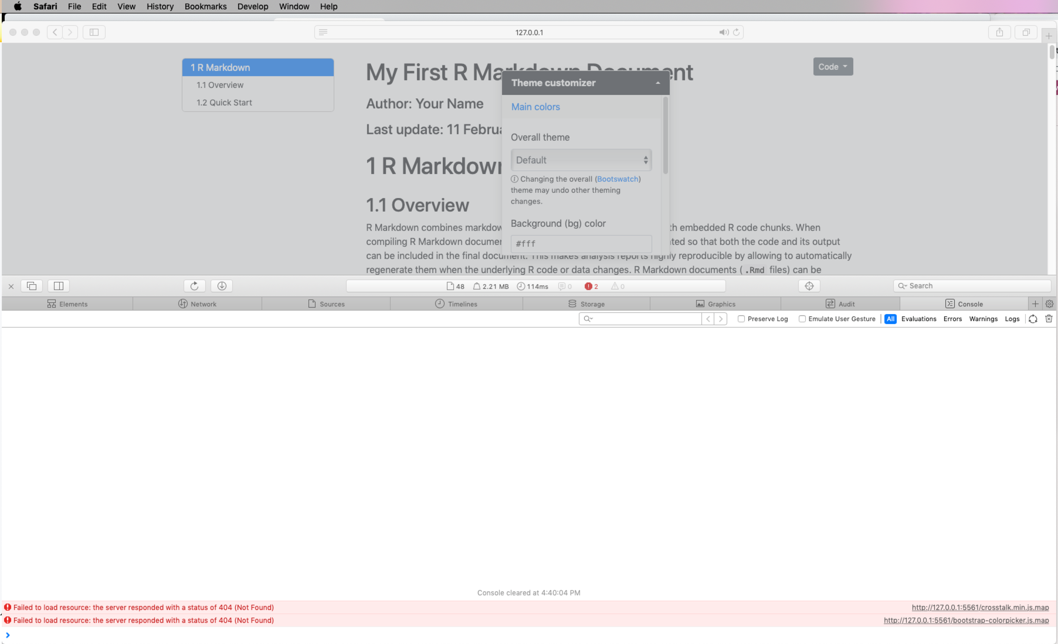
Safari throws console error loading rmarkdown file with interactive themer

[MadhulikaTanuboddi]

1. Run the attached rmarkdown file using rmarkdown::run()
2. Open the rmd on safari
3. Check the dev console on the browser

I see the following error.

Rmd example:

My First R Markdown Document using bslib

---
title: "My First R Markdown Document" 
author: "Author: Your Name"
date: "Last update: `r format(Sys.time(), '%d %B, %Y')`" 
runtime: shiny
output:
  html_document:
    theme: !expr bslib::bs_theme()
    toc: true
    toc_float:
        collapsed: true
        smooth_scroll: true
    toc_depth: 3
    fig_caption: yes
    code_folding: show
    code_download: true
    number_sections: true
---


```{r, echo = FALSE}
thematic::thematic_shiny(font = "auto")
bslib::bs_themer()
```

# R Markdown

## Overview

R Markdown combines markdown (an easy to write plain text format) with embedded
R code chunks. When compiling R Markdown documents, the code components can be
evaluated so that both the code and its output can be included in the final
document. This makes analysis reports highly reproducible by allowing to automatically
regenerate them when the underlying R code or data changes. R Markdown
documents (`.Rmd` files) can be rendered to various formats including HTML and
PDF. The R code in an `.Rmd` document is processed by `knitr`, while the
resulting `.md` file is rendered by `pandoc` to the final output formats
(_e.g._ HTML or PDF). Historically, R Markdown is an extension of the older
`Sweave/Latex` environment. Rendering of mathematical expressions and reference
management is also supported by R Markdown using embedded Latex syntax and
Bibtex, respectively.

## Quick Start

### Install R Markdown

```{r install_rmarkdown, eval=FALSE}
install.packages("rmarkdown")
```

### Initialize a new R Markdown (`Rmd`) script

To minimize typing, it can be helful to start with an R Markdown template and
then modify it as needed. Note the file name of an R Markdown scirpt needs to
have the extension `.Rmd`. Template files for the following examples are available 
here:

+ R Markdown sample script: [`sample.Rmd`](https://raw.githubusercontent.com/tgirke/GEN242/gh-pages/_vignettes/07_Rbasics/sample.Rmd)
+ Bibtex file for handling citations and reference section: [`bibtex.bib`](https://raw.githubusercontent.com/tgirke/GEN242/gh-pages/_vignettes/07_Rbasics/bibtex.bib)

Users want to download these files, open the `sample.Rmd` file with their preferred R IDE 
(_e.g._ RStudio, vim or emacs), initilize an R session and then direct their R session to 
the location of these two files.


### Metadata section

The metadata section (YAML header) in an R Markdown script defines how it will be processed and 
rendered. The metadata section also includes both title, author, and date information as well as 
options for customizing the output format. For instance, PDF and HTML output can be defined 
with `pdf_document` and `html_document`, respectively. The `BiocStyle::` prefix will use the
formatting style of the [`BiocStyle`](http://bioconductor.org/packages/release/bioc/html/BiocStyle.html) 
package from Bioconductor.

```
 ---
title: "My First R Markdown Document"
author: "Author: First Last"
date: "Last update: `r format(Sys.time(), '%d %B, %Y')`"
output:
  BiocStyle::html_document:
    toc: true
    toc_depth: 3
    fig_caption: yes

fontsize: 14pt
bibliography: bibtex.bib
 ---
```

### Render `Rmd` script

An R Markdown script can be evaluated and rendered with the following `render` command or by pressing the `knit` button in RStudio.
The `output_format` argument defines the format of the output (_e.g._ `html_document`). The setting `output_format="all"` will generate 
all supported output formats. Alternatively, one can specify several output formats in the metadata section as shown in the above example.

```{r render_rmarkdown, eval=FALSE, message=FALSE}
rmarkdown::render("sample.Rmd", clean=TRUE, output_format="html_document")
```

The following shows two options how to run the rendering from the command-line.

```{sh render_commandline, eval=FALSE, message=FALSE}
$ Rscript -e "rmarkdown::render('sample.Rmd', clean=TRUE)"
```

Alternatively, one can use a Makefile to evaluate and render an R Markdown
script. A sample Makefile for rendering the above `sample.Rmd` can be
downloaded [`here`](https://raw.githubusercontent.com/tgirke/GEN242/gh-pages/_vignettes/07_Rbasics/Makefile).
To apply it to a custom `Rmd` file, one needs open the Makefile in a text
editor and change the value assigned to `MAIN` (line 13) to the base name of
the corresponding `.Rmd` file (_e.g._ assign `systemPipeRNAseq` if the file
name is `systemPipeRNAseq.Rmd`).  To execute the `Makefile`, run the following
command from the command-line.

```{sh render_makefile, eval=FALSE, message=FALSE}
$ make -B
```

### R code chunks

R Code Chunks can be embedded in an R Markdown script by using three backticks
at the beginning of a new line along with arguments enclosed in curly braces
controlling the behavior of the code. The following lines contain the
plain R code. A code chunk is terminated by a new line starting with three backticks.
The following shows an example of such a code chunk. Note the backslashes are
not part of it. They have been added to print the code chunk syntax in this document.

```
	```\{r code_chunk_name, eval=FALSE\}
	x <- 1:10
	```
```

The following lists the most important arguments to control the behavior of R code chunks:

+ `r`: specifies language for code chunk, here R
+ `chode_chunk_name`: name of code chunk; this name needs to be unique
+ `eval`: if assigned `TRUE` the code will be evaluated
+ `warning`: if assigned `FALSE` warnings will not be shown
+ `message`: if assigned `FALSE` messages will not be shown
+ `cache`: if assigned `TRUE` results will be cached to reuse in future rendering instances
+ `fig.height`: allows to specify height of figures in inches
+ `fig.width`: allows to specify width of figures in inches

For more details on code chunk options see [here](https://www.rstudio.com/wp-content/uploads/2015/03/rmarkdown-reference.pdf).


### Learning Markdown

The basic syntax of Markdown and derivatives like kramdown is extremely easy to learn. Rather
than providing another introduction on this topic, here are some useful sites for learning Markdown:

+ [Markdown Intro on GitHub](https://guides.github.com/features/mastering-markdown/)
+ [Markdown Cheet Sheet](https://github.com/adam-p/markdown-here/wiki/Markdown-Cheatsheet)
+ [Markdown Basics from RStudio](http://rmarkdown.rstudio.com/authoring_basics.html) 
+ [R Markdown Cheat Sheet](http://www.rstudio.com/wp-content/uploads/2015/02/rmarkdown-cheatsheet.pdf)
+ [kramdown Syntax](http://kramdown.gettalong.org/syntax.html)

### Tables

There are several ways to render tables. First, they can be printed within the R code chunks. Second, 
much nicer formatted tables can be generated with the functions `kable`, `pander` or `xtable`. The following
example uses `kable` from the `knitr` package.

```{r kable}
library(knitr)
kable(iris[1:12,])
```

A much more elegant and powerful solution is to create fully interactive tables with the [`DT` package](https://rstudio.github.io/DT/). 
This JavaScirpt based environment provides a wrapper to the DataTables library using jQuery. The resulting tables can be sorted, queried and resized by the
user. 

```{r dt}
library(DT)
datatable(iris, filter = 'top', options = list(
  pageLength = 100, scrollX = TRUE, scrollY = "600px", autoWidth = TRUE
))
```

### Figures

Plots generated by the R code chunks in an R Markdown document can be automatically 
inserted in the output file. The size of the figure can be controlled with the `fig.height`
and `fig.width` arguments.

```{r some_jitter_plot, warning=FALSE}
library(ggplot2)
renderPlot({
  dsmall <- diamonds[sample(nrow(diamonds), 1000), ]
  ggplot(dsmall, aes(color, price/carat)) + geom_jitter(alpha = I(1 / 2), aes(color=color))
})
```


### Inline R code

To evaluate R code inline, one can enclose an R expression with a single back-tick
followed by `r` and then the actual expression.  For instance, the back-ticked version 
of 'r 1 + 1' evaluates to `r 1 + 1` and 'r pi' evaluates to `r pi`.

### Mathematical equations

To render mathematical equations, one can use standard Latex syntax. When expressions are 
enclosed with single `$` signs then they will be shown inline, while 
enclosing them with double `$$` signs will show them in display mode. For instance, the following 
Latex syntax `d(X,Y) = \sqrt[]{ \sum_{i=1}^{n}{(x_{i}-y_{i})^2} }` renders in display mode as follows:

$$d(X,Y) = \sqrt[]{ \sum_{i=1}^{n}{(x_{i}-y_{i})^2} }$$