compute information gain in textmodel_nb
Hello,
A useful feature would be to add the information gain as defined p.17 of https://web.stanford.edu/~jurafsky/slp3/4.pdf. That would be a pretty useful metric.
What do you think? Thanks!
Hi @randomgambit , currently we already have textstat_entropy as a function, which supports the computation of entropy along both documents and features:
> textstat_entropy(dfm(data_corpus_inaugural))
1789-Washington 1793-Washington      1797-Adams  1801-Jefferson  1805-Jefferson
       7.770221        6.094922        7.754489        7.768814        7.953447
   1809-Madison    1813-Madison     1817-Monroe     1821-Monroe      1825-Adams
       7.608605        7.625116        7.982008        8.080853        7.838801
...
> textstat_entropy(dfm(data_corpus_inaugural), margin = 'features')
fellow-citizens              of             the          senate             and
      3.6849336       5.5333166       5.5327733       2.8159221       5.6547444
          house representatives               :           among    vicissitudes
      2.9139771       3.6163486       4.7401661       5.0918876       2.3219281
       incident              to            life              no           event
      2.5000000       5.6068178       5.3148646       5.2873975       3.0306391
...
The measure computed by textstat_entropy is the empirical analogue of
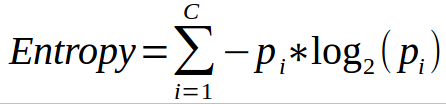 where Pi is the probability of document / feature appearing estimated with their proportion in the dfm.
May I clarify if this sufficient what you need, or do you refer to information gain from a word feature to evaluate feature importances in for a text classification model produced by textmodel_nb? (e.g. if fellow-citizens is included, what's the information gain relative to when it's excluded? )
If it is the latter, I am happy to help write the implementation.
But I think before I get started, it would be good to have @kbenoit 's input about whether this feature evaluation functionality we want to build into quanteda in the first place.
Hi @jiongweilua , yes I think it would be nice to have that feature importance metric for the naive bayes model. This is a very efficient classification algorithm and it would be interesting to be able to find out the most relevant words. One can do that by looking at the word likelihoods, but I am not sure its the optimal way to do (the likelihood are biased estimates)
This would be useful, and echoes quanteda/quanteda#1120. We have an influence() function that works on predicted textmodel_affinity objects, and this is similar, but would work on a textmodel_nb fitted object. We could call it gain() and it would output a word x class matrix (since this statistic is class-specific. Using the internal quantities from a fitted textmodel_nb object, it should be easy to compute.
OK, I've had a chance to investigate this a lot more now, and I think my comment above is wrong: G(w) is not a class-specific measure, but rather aggregates across classes. (That's the summation operator!) In 7fb520139960ca6ba98c38ebf3d09cd447b59eac I have significantly reimplemented the function. It's much simpler and relies on existing code, but very slow.
Why? Because I think that to compute the influence of a word, we have to compute P(c | \bar{w}) by recomputing the model for a w and not-w as features. This quantity is not the same as 1 - P(c | w).
In Jurafsky and Martin, they really do not devote much attention to G(w) and the one sentence where they describe w is based on the documents in which a word occurs - in other words, a binomial model. This is not how we would compute it for the multinomial model. In Yang and Pederson, which I added to the reference, there is a mention of m-ness (since features are not binary in a word count / multinomial model) but in typical CS fashion, no one bothers to clarify their notation or provide specifics.
I'm not at all sure that I have this right, and certain that there could be a more efficient implementation, but let's first clarify what the right answers should be.
Hi @kbenoit,
I haven't looked through your implementation, but in my implementation removed in 7fb5201,
-
The
overall = sum(initial_entropy),overall = colSums(conditional_entropy))andoverall = colSums(conditional_entropy_comp)are summation over the classes. So I don't think initially computing the class specific information gain is an issue. -
I am aware that
P(c | \bar{w}) =/= (1 - P(c|w)). In my implementation, here's how I did it and I think this is correct, at least for the binary class case.
# Defining \bar{w} as the complement of w, then P(\bar{w}) + P(w) = 1

P(c | \bar{w} )
= P(c ∩ \bar{w}) / P(\bar{w})            # Definition of conditional probability
= (P(c) - P(c ∩ w)) / P(\bar{w})         # P(c) =  P(c ∩ \bar{w}) + P (c  ∩ w)
= (P(c) - P(c ∩ w) / ( 1 - P(w))             # P(\bar{w}) =  1 - P(w}
= (P(c) - [P(w|c) * P(c)] ) / ( 1 - P(w))  # P(c ∩ w) = P(w|c) * P(c)

# Compute P(c ∩ w)
Pcintersectw <- object$PwGc * object$Pc
# Compute P(c ∩ \bar{w})
Pcintersectwcomp <- object$Pc - Pcintersectw
# Compute P(c | \bar{w} )  =  P(c ∩ \bar{w}) / ( 1 - P(w))
PcGwcomp <- t(t(Pcintersectwcomp) / as.vector(1-object$Pw))
- The main concern I have is that I am not sure if my implementation above generalises to the multinomial case. When writing my code I had a two-class test case at the back of my mind. I will comment on this issue if I find a formula that extends to the multinomial case, before I implement it.
That's fine, and feel free to revive your code. One commit before the one in which I killed it, I simplified the code a bit too.
I was thinking whether it makes sense to compute a binary, "in document or not" w / \bar{w} for NB models with a multinomial distribution. I'm not sure it does, although we certainly could for a model computed with distribution = "Bernoulli".
But a few hours of my attempting to read about the operational implementation of this model was not very clarifying. Maybe you will have better results.
I couldn't find papers online that documented the exact information gain scores for an open dataset, but came up with 2 alternative ideas for verifying our implementation, but unfortunately have not been very successful:
- Idea 1) Use this CMU problem set on feature selection for text classification to verify our implementation. See page 10 bullet point 3.
The solution suggests that our top 10 most important features should be a subset of a list of 50 they specified. But my code below only shows 3 out of the 10 appearing in that list of 50, which looks quite bad... One explanation is that, although followed the solution to only consider words with min 50 frequency, it is still possible that our preprocessing steps are not exactly indentical.
> setwd('/Users/luajiongwei/Downloads/emailspam/train')
> library(readtext)
> library(dplyr)
> text <- readtext(getwd())
> spam_or_not <- sapply(text$doc_id, function(x) startsWith(x,"spm"))
> spam_or_not[spam_or_not == TRUE] = 'SPAM'
> spam_or_not[spam_or_not == FALSE] = 'NORMAL'
> dfm_spam <- dfm(corpus(text),tolower =  TRUE, remove_punct = TRUE, remove = stopwords("english")) %>%
+     dfm_trim(min_termfreq = 50)
>
> trainingset <- dfm_spam
> trainingclass <- factor(spam_or_not)
> nb <- textmodel_nb(trainingset, y = trainingclass, prior = "docfreq")
>
> info_gain <- gain(nb)
>
> top_10_gain <- info_gain %>%
+     top_n(10, gain_overall) %>%
+     select(feature)
>
> top_50_answersheet <- strsplit(c("5599, 3d, abstract, abstracts, acquisition, advertise, aol, approaches, bills, bonus, capitalfm, chair,
+ chomsky, click, cognitive, committee, comparative, computational, context, customers, deadline, discourse, evidence, ffa, floodgate, grammar, grammatical, hundreds, income institute, investment, lexical, linguist, linguistic, linguistics, linguists, marketing, millions, multi-level, offshore, papers, parallel,
+ phonology, product, programme, remove, researchers, sales, secrets, sell, semantic, semantics, sessions,
+ structure, submissions, syntax, texts, theoretical, theory, translation, win, workshop"), split = ", ")
> top_50_answersheet <- top_50_answersheet[[1]] %>% as.vector()
>
> sapply(top_10_gain[[1]], function(x)  x %in% top_50_answersheet) %>% sum()
[1] 3
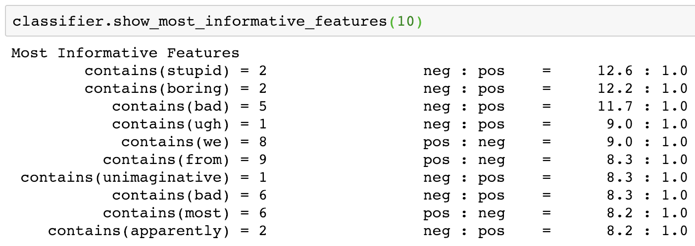
- Idea 2) Use the NLTK's implementation of
show_most_informative_featureson the nltk movie_reviews dataset. (from nltk.corpus import movie_reviews)
The trouble with this is that oddly, the nltk implementation of NaiveBayesClassifier takes feature counts as categorical variables rather than counts. And they don't seem to use the same information gain formula.
Python code available here
Any other suggestions about how I should proceed? @randomgambit @kbenoit
thats great. I think it is perfectly acceptable to send an email to Dan Juravsky asking whether he knows some paper that uses this metric. After all, he is the one mentioning it in his NLP book. He would also be very glad to know quanteda is citing his work.
Great ideas, and thanks @jiongweilua for the Python comparison, I will investigate both soon. Want to get the details really straight since I have plans to implement decision trees and SVMs for sparse text matrices and gain applies to both as well.
@randomgambit Of course! People contact me all the time with such questions, so you're right, it's a natural thing to do, and since the chapter is a draft anyway it is even akin to feedback. I will prepare and send something shortly.