Modify cosine angle functional form

[proteneer]

Our current harmonic angle oscillator has an option for cos_angles that we default to True. The original motivation for this was to avoid the numerical singularity that arises at 0 or 180 degrees. Most MD packages patch this behavior in odd ways, but it's really undesirable. So when I initially wrote the angle term, I adopted the gromos functional form of (cos(a)-cos(t))^2, which while it solves the issue at 0 and pi, it fails spectacularly for other values. After some debugging, (cos(a-t)-1)^2 is a much better approximation:

(red: original, green: gromos, current timemachine, purple: proposed)

[proteneer]

Nevermind, unfortunately my proposed functional form has a singularity as well:

[proteneer]

In terestingly enough, expressed as cartesian coordinates, the gromos form actually fits quite well, but the barriers may need to be rescaled.

[proteneer]

I think the gromos forcefield is actually fine, since the use of y=arccos(x), where -1<=x<=1 restricts the output to 0<=y<=pi:

[proteneer]

TL;DR: we should refit the force constants here with wrap-around considerations.

[proteneer]

A more simplified illustration:

[proteneer]

Note: a good zero-th order approximation is probably to just increase k by a factor of 2.

[maxentile]

Clarification: is the main concern:

1. force singularities that occur at a single point (dU/dx = nans when theta = theta_0 = 0 for example),
2. energy discontinuities due to non-periodic angular distance definition (theta - theta_0)^2

?

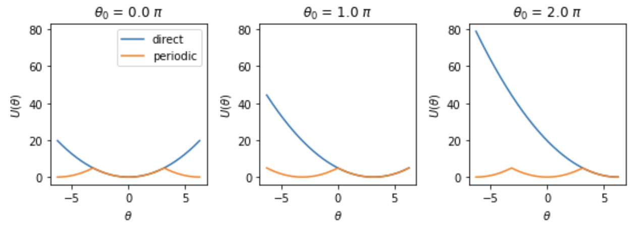
Possible workaround for 2: replace direct delta_theta = theta - theta_0 with periodic version:

import numpy as np
from jax import numpy as jnp
import matplotlib.pyplot as plt

theta_grid = np.linspace(-2 * np.pi, 2 * np.pi, 10000)

def direct_delta_theta(theta, theta_0):
    """does not satisfy d(theta, theta_0) = d(theta + 2pi, theta_0)"""
    return theta - theta_0

def periodic_delta_theta(theta, theta_0):
    """by analogy to PBC-compatible definition of delta_r"""
    # https://github.com/proteneer/timemachine/blob/451803e01afe6231147a0e6a3ca019d4aa5069d8/timemachine/potentials/jax_utils.py#L70-L77
    diff = theta - theta_0
    width = 2 * np.pi
    return diff - (width * jnp.floor(diff / width + 0.5))

def u_direct(theta, theta_0=0, k=1.0):
    return 0.5 * k * direct_delta_theta(theta, theta_0)**2

def u_periodic(theta, theta_0=0, k=1.0):
    return 0.5 * k * periodic_delta_theta(theta, theta_0)**2

plt.figure(figsize=(8,3))
ax = None
for i, theta_0 in enumerate([0, np.pi, 2*np.pi]):
    ax = plt.subplot(1, 3, i+1, sharey=ax)
    plt.title(rf'$\theta_0$ = {theta_0/np.pi} $\pi$')
    #theta_grid = np.linspace(theta_0 - 2 * np.pi, theta_0 + 2* np.pi, 10000)
    plt.plot(theta_grid, u_direct(theta_grid, theta_0=theta_0), label='direct')
    plt.plot(theta_grid, u_periodic(theta_grid, theta_0=theta_0), label='periodic')
    plt.xlabel(r'$\theta$'); plt.ylabel(r'$U(\theta)$')
    if i == 0: plt.legend()
plt.tight_layout()

Doesn't solve the problem of the forces being discontinuous at theta = theta_0 +/- pi, but this might be of limited practical concern when k is large.

[maxentile]

(Tangent: May be worth looking at numerical stability considerations for other angular distributions such as the Von Mises distribution, e.g. in Stan https://mc-stan.org/docs/2_22/functions-reference/von-mises-distribution.html or Mitsuba https://www.mitsuba-renderer.org/devblog/2012/07/numerically-stable-sampling-of-the-von-mises-fisher-distribution-on-s2-and-other-tricks/ )

[proteneer]

The main concern is:

1. force singularities that occur at a single point (dU/dx = nans when theta = theta_0 = 0 for example),

There are no discontinuities in the energy in any of the above functional forms.

[maxentile]

There are no discontinuities in the energy in any of the above functional forms.

Oh! Shoot -- you're right. (Assumed there would be a discontinuity since theta - theta_0 is not periodic as a function of theta, but I do not observe energy discontinuities of U as a function of conf (must be mitigated by the way theta is computed from conf -- will revisit more carefully sometime)... )

Sorry -- carry on!

[maxentile]

For future reference, these were points of my confusion:

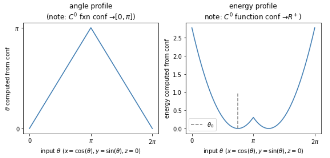
• Forgot the domain of theta here is [0, pi] not [0, 2pi] (or arbitrary [x, x + 2pi]). It is also computed as a continuous function of conf. The functional form U(theta) here only needs to be safe for theta in [0, pi], not over the larger intervals plotted above.
• The discontinuity in the forces is not just that forces become undefined / nan at a single point, but also that some force components point in opposite directions as conf approaches theta(conf) == pi in different ways

Plot of angle(conf) and energy(conf):

from timemachine.potentials.bonded import harmonic_angle
import numpy as np
from jax import numpy as jnp
from jax.numpy.linalg import norm
import matplotlib.pyplot as plt

def compute_theta(conf):
    """https://github.com/proteneer/timemachine/blob/451803e01afe6231147a0e6a3ca019d4aa5069d8/timemachine/potentials/bonded.py#L213-L225"""
    
    x_a, x_b, x_c = conf
    
    v_ab = x_a - x_b
    v_cb = x_c - x_b
    theta = jnp.arccos(jnp.dot(v_ab, v_cb) / (norm(v_ab) * norm(v_cb)))
    
    return theta


def U_angle(conf, theta_0=0, k=1, cos_angles=True):
    assert len(conf) == 3
    
    angle_idxs = jnp.array([[0,1,2]])
    params = jnp.array([[k, theta_0]])
    
    unused_required_params = dict(
        box=None,
        lamb=None,
    )
    return harmonic_angle(conf, params=params, angle_idxs=angle_idxs, cos_angles=cos_angles, **unused_required_params)


# scan out confs in a circle on the x-y plane
theta_grid = np.linspace(0, 2 * np.pi, 1000)


def conf_from_angle(theta):
    """theta in R -> conf in R^3x3"""
    a = np.array([1, 0, 0])
    b = np.array([0, 0, 0])
    c = np.array([np.cos(theta), np.sin(theta), 0])
    conf = np.array([a, b, c])
    return conf


confs = [conf_from_angle(theta) for theta in theta_grid]

# compute energy as a function of theta, for theta_0 = 3pi/4
theta_0 = 0.75 * np.pi

theta_profile = np.array([compute_theta(conf) for conf in confs])
U_profile = np.array([U_angle(conf, theta_0=theta_0, cos_angles=False) for conf in confs])

# plot angle profile
plt.figure(figsize=(8,4))
plt.subplot(1,2,1); plt.title('angle profile\n' + r'(note: $C^0$ fxn conf $\to [0, \pi$])')
plt.plot(theta_grid, theta_profile)
plt.xlabel(r'input $\theta$ $(x=\cos(\theta), y=\sin(\theta), z=0)$')
plt.ylabel(r'$\theta$ computed from conf')
plt.xticks([0, np.pi, 2 * np.pi], ['0', r'$\pi$', r'$2\pi$', ])
plt.yticks([0, np.pi], ['0', r'$\pi$'])

# plot energy profile
plt.subplot(1,2,2); plt.title('energy profile\n' + r'note: $C^0$ function conf $\to R^+$)')
plt.plot(theta_grid, U_profile)
plt.vlines(theta_0, 0, 1, linestyles='--', color='grey', label=r'$\theta_0$')
plt.xlabel(r'input $\theta$ $(x=\cos(\theta), y=\sin(\theta), z=0)$')
plt.ylabel(r'energy computed from conf')
plt.xticks([0, np.pi, 2 * np.pi], ['0', r'$\pi$', r'$2\pi$', ])
plt.legend()

plt.tight_layout()

dudx(conf_a), dudx(conf_b) near discontinuity:

distance(conf_a, conf_b) 0.001999999666666463
dudx(conf_a) [[ 0.0000000e+00 -8.0324775e-01  0.0000000e+00]
 [ 7.3242188e-04  1.6064951e+00  0.0000000e+00]
 [-7.3242188e-04 -8.0324739e-01  0.0000000e+00]]
dudx(conf_b) [[ 0.0000000e+00  8.0324775e-01  0.0000000e+00]
 [ 7.3242188e-04 -1.6064951e+00  0.0000000e+00]
 [-7.3242188e-04  8.0324739e-01  0.0000000e+00]]

# some force components point in opposite directions as theta approaches pi
from jax import grad

conf_a = conf_from_angle(np.pi - 0.001)
conf_b = conf_from_angle(np.pi + 0.001)

dudx_a = grad(U_angle)(conf_a, theta_0=theta_0, cos_angles=False)
dudx_b = grad(U_angle)(conf_b, theta_0=theta_0, cos_angles=False)

print('distance(conf_a, conf_b)', np.linalg.norm(conf_a - conf_b))
print('dudx(conf_a)', dudx_a)
print('dudx(conf_b)', dudx_b)

[maxentile]

Closed by https://github.com/proteneer/timemachine/pull/1271