SGTK
 SGTK copied to clipboard
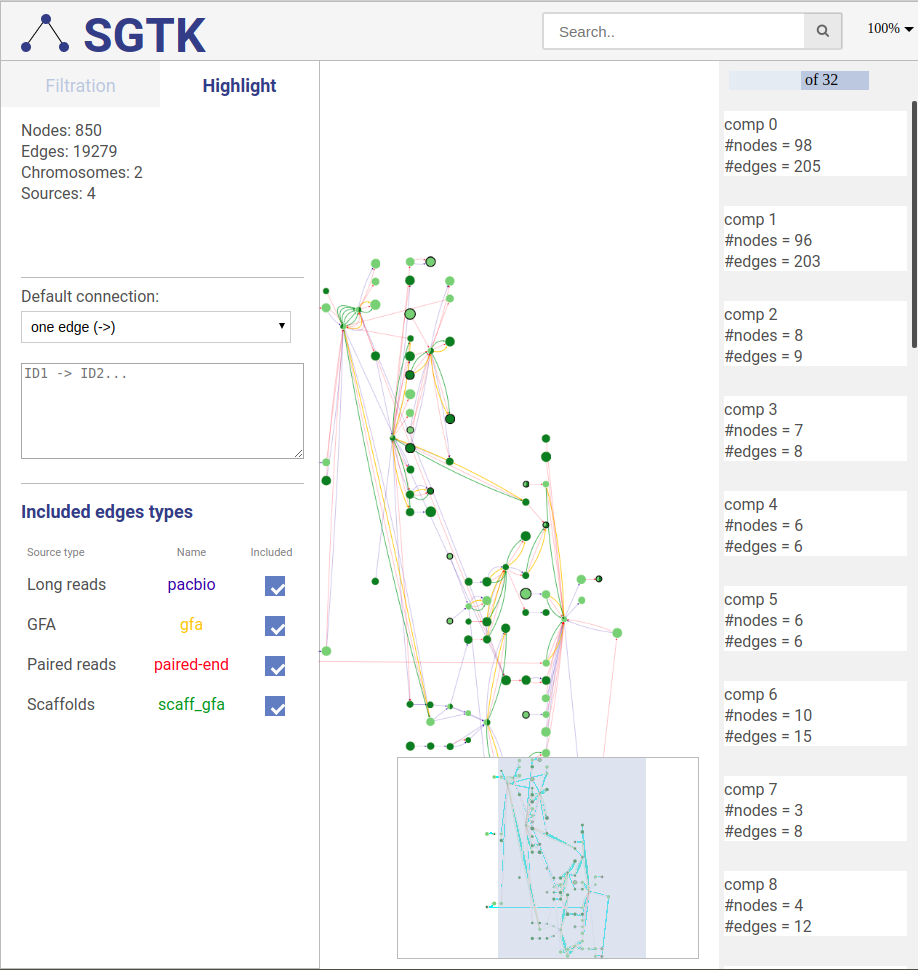
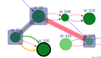
Example of SGTK application for E.coli dataset:
-
About SGTK
-
Installation
-
Running SGTK
3.1. Command line options
3.2. Command line examples
3.3. Output
3.4. Example dataset
-
Visualization
4.1. Getting started
4.2. Genome browser layout
4.3. Free layout mode
4.4. Customizing visualization
4.5. Highlighting paths
4.6. Understanding visualization
4.7. Navigation
-
RNA-Seq scaffolder
-
References
-
Feedback and bug reports
Quick start
Installation
The easiest way is to install SGTK via conda:
conda install -c olga24912 -c conda-forge -c bioconda sgtk
Alternatively, you can either download SGTK binaries or compile it by yourself. The latest release can be downloaded here.
To run SGTK graph construction you need to install Biopython. If you wish to construct scaffold graph using DNA sequences (long reads, read-pairs, scaffolds or reference genome) you will need minimap2. If you want to use RNA-Seq reads you will need STAR aligner. All packages are automatically installed if you use conda.
Graph visualization is stored in HTML format and can be viewed in any web browser.
Running SGTK
To construct and visualize the scaffold graph based on contigs run
sgtk.py -c <contigs.fa> [--fr <left_pe.fq> <right_pe.fq>]  \
[--rf <left_mp.fq> <right_mp.fq>] [--long <pacbio.fq/ont.fq>] \
[--ref <genome.fa>] [-s <scaffolds.fa>] \
-o <output_dir>
Alternatively, instead of <contigs.fa>, one may provide GFA
sgtk.py --gfa <graph.gfa> -o <output_dir> [options]
or FASTG file
sgtk.py --fastg <graph.fastg> -o <output_dir> [options]
Once graph construction is finished, open
<output_dir>/main.html
in you favourite browser (but better use Chrome). If you intend to transfer the visualization, do not forget to include <output_dir>/scripts/ folder.
1. About SGTK
SGTK – Scaffold Graph ToolKit – is a tool for construction and interactive visualization of scaffold graph. Scaffold graph is a graph where vertices are contigs, and edges represent links between them. Contigs can provided either in FASTA format or as the assembly graph in GFA/GFA2/FASTG format. Possible linkage information sources are:
- paired reads
- long reads
- paired and unpaired RNA-seq reads
- scaffolds
- assembly graph in GFA1, GFA2, FASTG formats
- reference sequences
SGTK produces a JavaScript-based HTML page that does not require any additional libraries and can be viewed in a regular web browser. Although it was tested in Chrome, FireFox, Opera and Safari, Chrome is preferred.
However, to construct a graph using SGTK application you will need a 64-bit Linux system or Mac OS and Python 3. If you plan to construct graph using sequencing data or reference genome you will also need the following aligners (installed automatically if you use conda):
- minimap2 for aligning DNA sequences (long reads, read-pairs, scaffolds or reference genome)
- STAR for mapping RNA-Seq
More details are provided below.
2. Installation
Conda and pre-compiled binaries
The easiest way is to install SGTK via conda:
conda install -c olga24912 -c conda-forge -c bioconda sgtk
This command installs all required dependencies, including minimap2 and STAR aligner.
Alternatively, you can can either download binaries, or download source code and compile it yourself. In this case you need to install Biopython, minimap2 and STAR aligner by yourself.
SGTK has precompiled binaries for Linux and MacOS. The latest builds can be downloaded for the GitHub page.
Once unpacked, SGTK is ready to use. You may also consider adding SGTK installation directory to the PATH variable.
Compiling SGTK source code
To compile SGTK by yourself you will need the following libraries to be pre-installed:
- gcc (version 5 or higher) / Clang (version 3.6 or higher)
- cmake (version 3.5 or higher)
- zlib
- Threads
- Biopython
- Boost
- SEQAN (version 2.4 or higher)
If you meet these requirements, you can download the SGTK source code here. Unpack the archive and build it with the following script:
./compile.sh
SGTK will be built in the directory ./bin. If you wish to install SGTK into another directory, you can specify the full path of destination folder by running:
PREFIX=<destination_dir> ./compile.sh
for example:
PREFIX=/usr/local ./compile.sh
which will install SGTK into /usr/local/bin. We also suggest adding SGTK installation directory to the PATH variable.
After installation you will get the following files in the installation directory:
-
sgtk.py(main executable script for visualization scaffold graph) -
rna_scaffolder.py(main executable script for building scaffolds using RNA-Seq data) -
buildApp(graph construction module) -
filterApp(graph simplification and building scaffolds module) -
mergeGraph(graph merging module) -
readSplitter(module for splitting RNA-seq reads) -
mainPage.html(main HTML page for visualization) -
scripts/(folder containing JS necessary for visualization)
3. Running SGTK
SGTK requires at least one set of contigs, which can be provided as usual FASTA file, or as the assembly graph in FASTG/GFA/GFA2 format.
To run scaffold graph visualization from the command line, type
sgtk.py [options]
Note that we assume that SGTK installation directory is added to the PATH variable (otherwise provide full path to SGTK executable: <installation dir>/sgtk.py).
3.1. Command line options
All input options are capable of taking only a single or a pair of files if specified. To provide multiple files use the same option again (e.g. -c contigs1.fa -c contigs2.fa). See more in the examples.
-h (or --help)
Print help.
-o (or --local_output_dir) <output_dir>
Output directory. The default output directory is "./".
-c (or --contig) <file_name>
File with contigs in FASTA format. You can provide a few contigs files (each one must be preceded by the option, i.e. -c contigs1.fa -c contigs2.fa), in this case they will be merged together. Make sure that all contigs have different names.
--fastg <file_name>
File with assembly graph in FASTG format. Edges will be treated as input contigs, the graph itself will be visualized.
--gfa <file_name>
File with assembly graph in GFA1 format. Edges will be treated as input contigs, the graph itself and scaffolds (paths) will be visualized.
--gfa2 <file_name>
File with assembly graph in GFA2 format. If segments are present they will be treated as input contigs. Otherwise, file with contigs must be provided. The graph with gap edges will be visualized. Note, that GFA2 is supported only partially.
Linkage sources
--fr <file_name_1> <file_name_2>
A pair of files with left and right reads for paired-end/mate-pair DNA library with forward-reverse orientation in FASTQ/FASTA format.
Input reads are aligned to contigs using minimap2.
--rf <file_name_1> <file_name_2>
A pair of files with left and right reads for paired-end/mate-pair DNA library with reverse-forward orientation in FASTQ/FASTA format.
--ff <file_name_1> <file_name_2>
A pair of files with left and right reads for paired-end/mate-pair DNA library with forward-forward orientation in FASTQ/FASTA format.
--fr_sam <file_name_1> <file_name_2>
A pair of files with left and right reads alignments in SAM/BAM format for paired-end/mate-pair DNA library with forward-reverse orientation.
--rf_sam <file_name_1> <file_name_2>
A pair of files with left and right reads alignments in SAM/BAM format for paired-end/mate-pair DNA library with reverse-forward orientation.
--ff_sam <file_name_1> <file_name_2>
A pair of files with left and right reads alignments in SAM/BAM format for paired-end/mate-pair DNA library with forward-forward orientation.
--long <file_name>
File with PacBio/Oxford Nanopore reads in FASTQ/FASTA format, which will be aligned using minimap2:
--rna-p <file_name_1> <file_name_2>
A pair of files with left and right reads for paired-end RNA-Seq library in FASTQ/FASTA format. Reads will be aligned to the contigs independently (using STAR).
--rna-s <file_name>
File for single RNA-Seq reads in FASTQ/FASTA format. Reads will be split into two parts and then aligned to the contigs using STAR.
--ref <file_name>
File with reference genome in FASTA format. In case if several files are provided (each file must be preceded by the option, i.e. --ref genome1.fa --ref genome2.fa)
they will be merged together and chromosomes names will be changed depending on the files names (useful for metagenomic datasets). Reference sequences are mapped using minimap2.
-s (or --scaffolds) <file_name>
File with scaffolds in FASTA format, which will be aligned to the contigs using minimap2.
--scg <file_name>
File with connection list. Each line in such file represents a single connection:
(CONTIG_1 ORIENTATION_1) (CONTIG_2 ORIENTATION_2) WEIGHT DISTANCE "COMMENTS"
For example:
(contig1 -) (contig3 +) 32.5 1168 "this is a reliable connection"
--scafinfo <file_name>
File with scaffolds in INFO format (introduced in Rascaf). In INFO format each line describes a scaffold in the following format:
>SCAFFOLD_NAME (CONTIG_NAME_1 CONTIG_ID_1 ORIENTATION_1) (CONTIG_NAME_2 CONTIG_ID_2 ORIENTATION_2)
For example:
>scaffold0001 (contig1 1 +) (contig3 3 -) (contig2 2 -) (contig8 8 +)
--label <label1 label2 ...>
List of labels used in visualization for libraries in given order. Labeling is not available for reference sequences.
--color <color1 color2 ...>
List of colors used in visualization for libraries in given order. Color can be provided in any format supported by HTML in double quotes, e.g. as word ("reb", "blue", etc) or as hexadecimal number ("#ff0000"). Coloring is not available for reference sequences.
Scaffold graph in the internal format
It is also possible to specify scaffold graph in the internal SGTK format with
--gr <file_name>
If other linkage sources are provided, they will be merged together into one scaffold graph.
Scaffold graph has the following format:
LIBS_DESCRIPTIONS
NODES_DESCRIPTIONS
EDGES_DESCRIPTIONS
The format for LIBS_DESCRIPTIONS:
NUMBER_OF_LIBS
(l LIB_ID LIB_COLOR LIB_NAME LIB_TYPE) * NUMBER_OF_LIBS
Where LIB_TYPE = {CONNECTION | LONG | DNA_PAIR | RNA_PAIR | GFA | GFA2 | FASTG | SCAFF}
The format for NODES_DESCRIPTIONS:
NUMBER_OF_NODES
(v NODE_ID NODE_NAME NODE_LEN) * NUMBER_OF_NODES
Format for EDGES_DESCRIPTIONS:
NUMBER_OF_EDGES
(e EDGE_ID NODE_ID_1 NODE_ID_2 LIB_ID WEIGHT DIST "COMMENTS") * NUMBER_OF_EDGES
For example:
1
l 0 #ff0000 lib_name DNA_PAIR
4
v 0 node_0 20132
v 1 node_0-rev 20132
v 2 node_1 20400
v 3 node_1-rev 20400
2
e 0 0 2 0 32.5 200 "some extra info"
e 1 3 1 0 32.5 200
3.2. Command line examples
Let's say our dataset consists of:
- A set of contigs (
contigs.fa) - Illumina paired-end lib (
pe1.fq, pe2.fq) - Illumina mate-pair lib (
mp1.fq, mp2.fq) - PacBio reads (
filtered_subreads.fq) - Several sets of scaffolds generated by different tools (
scaffolds1. fa, scaffolds2.fa, scaffolds3.fa) - Reference genome splitted into separate chromosomes (
chr1.fa, chr2.fa, chr3.fa)
In addition you'd like to set the colors and labels for each linkage source.
Then the command line for launching SGTK would look like:
python3 sgtk.py -c contigs.fa \
--ref chr1.fa --ref chr2.fa --ref chr3.fa \
--fr pe1.fq pe2.fq  --rf mp1.fq mp2.fq  --long filtered_subreads.fq \
-s scaffolds1.fa  -s scaffolds2.fa  -s scaffolds3.fa \
--label PE MP PacBio Tool1 Tool2 Tool3 \
--color "#ff0000" "#ffff00" "#00ff00" "#ff00ff" "#ffcccc" "#ccff00" \
-o output_dir
3.3. Output
SGTK stores all output files in <output_dir> , which is set by the user.
-
<output_dir>/main.htmlmain file for graph visualization. -
<output_dir>/scripts/files with scaffold graph description, which are needed formain.html. If you intend to transfer the generated visualization to another machine, do not forget to include this folder.
Open main.html in any browser to see visualisation. Chrome is preferred.
3.4. Example dataset
SGTK comes with toy dataset, on which you can test your installation:
- contigs (
share/test_dataset/contigs.fasta) - Illumina paired-end library (
share/test_dataset/read_1.fasta, share/test_dataset/read_2.fasta) - assembled scaffolds (
share/test_dataset/scaf.info) - reference genome (
share/test_dataset/ref.fasta)
To test the toy data set, you can run the following command from the SGTK bin directory:
python3 sgtk.py -c ../share/test_dataset/contigs.fasta \
--fr ../share/test_dataset/read_1.fasta ../share/test_dataset/read_2.fasta \
--scafinfo ../share/test_dataset/scaf.info \
--ref ../share/test_dataset/ref.fasta \
-o output
If you would like to set labels and colors, you need to set labels and colors for all libraries in order of definition
python3 sgtk.py -c ../share/test_dataset/contigs.fasta \
--ref ../share/test_dataset/ref.fasta \
--fr ../share/test_dataset/read_1.fasta ../share/test_dataset/read_2.fasta \
--scafinfo ../share/test_dataset/scaf.info \
--label PE scaffolds \
--color "#0000ff" "#00ff00" \
-o output
In addition, you can try SGTK visualization examples which we uploaded here. You can also clone the repository:
git clone https://github.com/olga24912/SGTK.git
cd SGTK
and open ./resources/E.coli/main.html in browser.
This example is constructed from E.coli paired-end reads and pacbio reads. Contigs and scaffolds were taken from GFA file, reference genome was also provide.
4. Visualization
4.1. Getting started
After the graph is constructed and the web page is generated, you can open main.html in a web browser (we recommended to use Chrome, however it also was tested in FireFox, Opera and Safari).
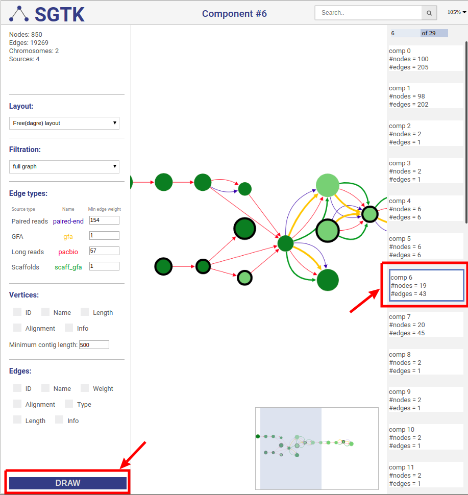
You can click on the DRAW button at the bottom of the left panel and choose a component for visualization at the right panel. By default the full graph is separated into components. If a component contains more than 100 nodes and 200 edges it will be randomly split into parts and visualized independently.
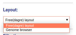
SGTK has two layout modes: (i) free layout and (ii) genome browser. Free layout option is available for all kinds of data. In genome browser layout contigs are aligned along reference chromosomes, which makes it available only if the reference is provided.
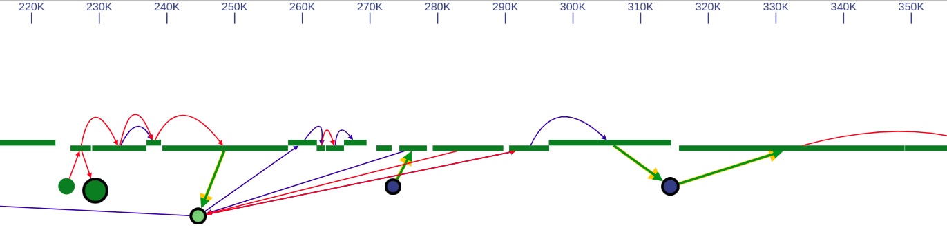
4.2. Genome browser layout
In the genome browser mode, vertices of the scaffold graph are displayed as rectangles placed along the reference, lengths of which are proportional to the contigs sizes. Short nodes with adjacent edges are hidden and rendered only when zoomed in.
4.3. Free layout mode
In case of free layout you can choose one of several filtration options. Once new visualization parameters are set, click the DRAW button and choose the component.
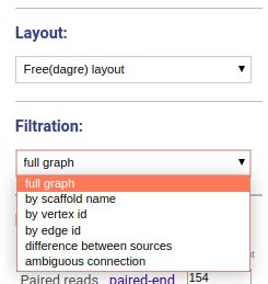
Drawing the entire graph
No filtering is applied, the full graph will be visualized. Graph will be randomly split into the components and all components will be visualized independently.
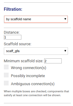
Drawing graph along scaffold
This options allows to visualize the graph around selected scaffolds. You may choose the distance from the scaffold hits and which scaffolds set you would like to visualize. You may also filter scaffolds based on their minimal length and other properties:
- Scaffolds containing wrong connections (i.e. disagreed with the reference genome)
- Possibly incomplete scaffolds
- Scaffolds with ambiguous connections
When multiple boxes are checked, components that satisfy at least one parameter will be shown.
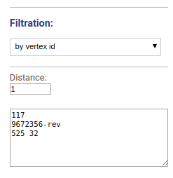
Drawing graph around vertices
Visualizes the vicinity of chosen vertices. Vertices names or ids are specified separated by space, new line or comma.
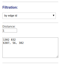
Drawing graph around edges
Visualizes the vicinity of chosen edges. Edges names or ids are specified separated by space, new line or comma.
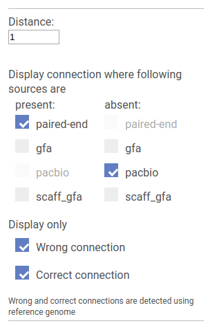
Detecting incorrect connections
In this mode SGTK allows to find the difference between linkage sources.
Wrong and Correct checkboxes allow to set whether we are interested in connection that are supported by the reference genome or not. If the reference genome is not provided all connections are treated as wrong.
Below, for each source type there is a pair of checkboxes: Present and Absent. SGTK locates pairs of vertices that are connected by all sources marked as Present and are not connected by any of the sources marked as Absent.
Displaying ambiguous connections
Visualizes the local area of the specified size for vertices that have more than one incoming or outgoing edge.
4.4. Customizing visualization
Connection sources
Information about connections sources is displayed at the left as displayed below.
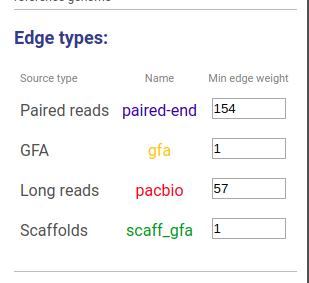
Supported connection types are:
- Long reads: long reads such as Pacbio or Oxford Nanopores
- Paired reads: mate-pairs and paired-end DNA short reads
- RNA-Seq (paired): paired-end RNA-Seq
- RNA-Seq (single): RNA-Seq single reads
- Scaffold
- GFA: assembly graph connections from GFA file
- GFA2: assembly graph connections from GFA2 file
- FASTG: assembly graph connections from FASTG file
- Connection: from file with connections list
The third column shows sources names, text color is the same as color of edges. The last column represents weight threshold for this source, which can be set by user. To apply changes click DRAW button.
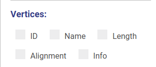
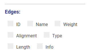
Hiding and displaying information
Using controls displayed below you can set which properties will be shown near vertices and edges. These changes will be applied automatically without redrawing.
Minimum contig length
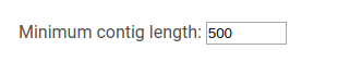
You can set up threshold for visualizing nodes. Note, that when visualizing nodes along scaffolds contigs shorter than the threshold still will be displayed.
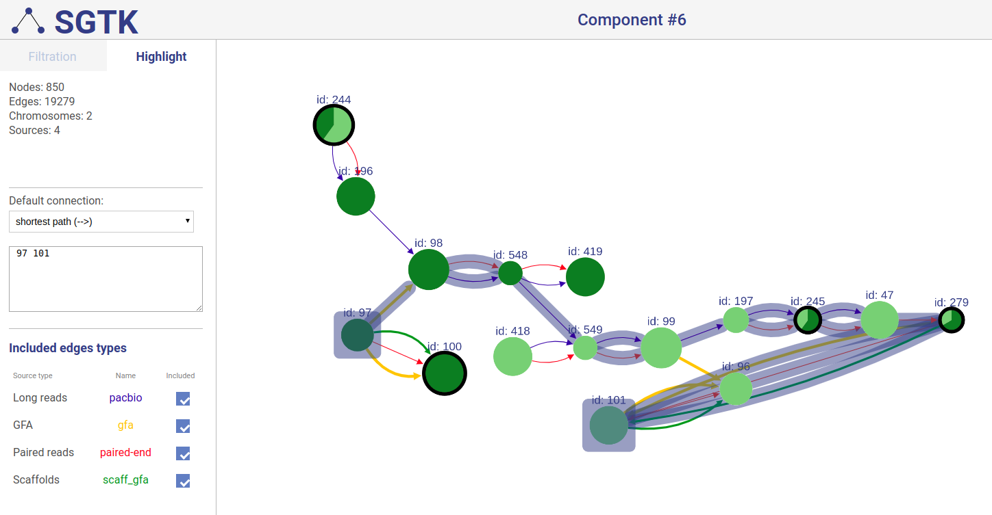
4.5. Highlighting paths
To ease the analysis, you can also highlight vertices, edges, paths and entire scaffolds. To use this functionality, switch to highlight tab (top left).
Highlighted path description
Path description
To highlight a set of edges or vertices, one needs to specify them in the text box using simple description script.
There are following types of highlight description are currently supported:
-
scaffold_name- scaffold name to highlight; will highlight all vertices and connections corresponding to this scaffold. -
a- contig name or contig id to highlight the corresponding vertex. -
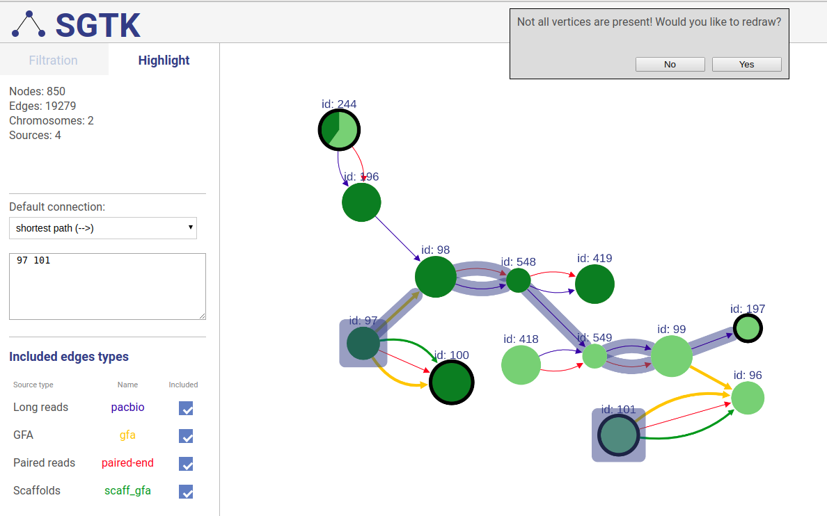
a --> b- will find and highlight the shortest path between vertices a and b. -
a -> b- highlight vertices a and b and all connections between them. -
a; b- highlight vertices a and b without highlighting any connections between them. -
a -eid> b- highlight vertices a and b, as well as edge eid if it connects these two vertices. -
a bin this case the default connection type between vertices a and b will be used (see below).
Each vertex is specified by corresponding contig name or id.
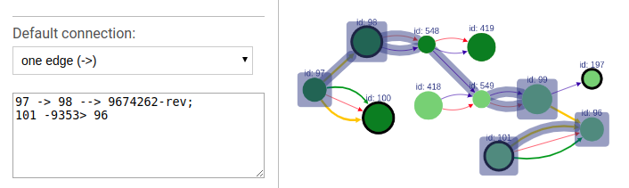
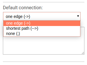
Default connection
To choose the default connection type use the appropriate drop-down menu. Available types are: path, edge or none.
Extending highlighted paths
To extend currently highlighted path, you can hold your left mouse button while pointing on the vertex of interest.
Extending displayed component
If a path or a set of vertices/edges chosen to be highlighted is not entirely displayed in the current view, you will be prompted about extending the view and showing absent vertices.
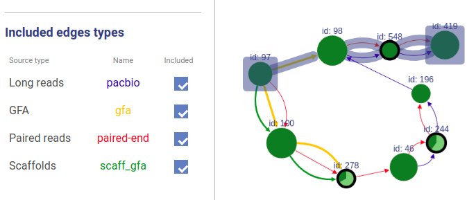
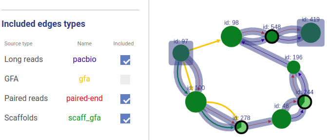
Included connection sources
You can also choose which connection types will be highlighted.
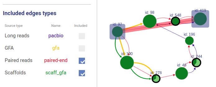
Missing edges
If a user asks to highlight an edge between two vertices that are not connected, a fake edge will be drawn between them and highlighted with red color (instead of typical blue highlight). Such option can be useful, for example, when comparing scaffolds obtained with different methods.
4.6. Understanding visualization
Below we provide brief information on how interprete SGTK visualization.
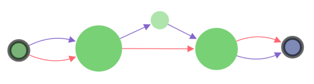
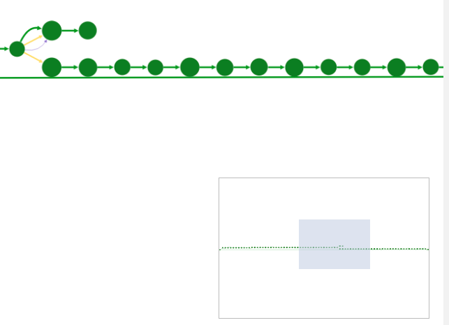
Vertices coloring
Colors of vertices correspond to alignment contigs on chromosomes.
Blue color means unaligned contig.

In case when a contig is aligned to more than one chromosome, the vertex is colored in sectors. Sector sizes represent the alignment fractions. Only top 3 alignments are shown.

Vertex size
Size of the vertex is proportional to the contig length in the logarithmic scale.
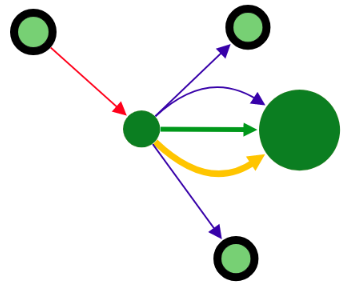
Edges width
Edges have different width depending on source type and visualization mode. The width is assigned in the following order (from thickest to thinnest):
- Currently visualized scaffold
- Connections from the assembly graph (GFA1, GFA2 or FASTG)
- Scaffolds connections
- All other connection types
Vertex with border
When a vertex has a black border, it means there are hidden adjacent edges, which are not shown at the current picture.
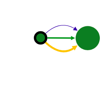
You can expand the vertex by clicking on this vertex and hidden connection will be shown.
In addition, the vertex can be removed by clicking on it with the right mouse button.
Pale nodes and edges
When a specific area is displayed (e.g. specified nodes, vertices, etc), focused elements have normal opacity, while the rest are drawn slightly transparent.
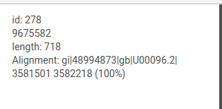
Information about edges and nodes
General information about the graph is shown at the top of the left panel.
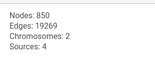
When the courson is pointed over a graph element, information about this node or edge will be displayed at the top of the left panel.
4.7. Navigation
View navigator
The view navigator (or "bird’s eye view") shows an overview of the graph. The blue rectangle indicated currently displayed part of the graph. It can be dragged with the mouse to view other part of graph.
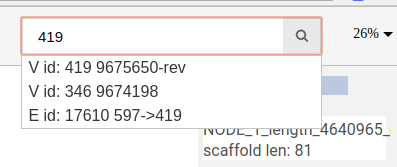
Search in free layout
You can search for nodes and edges by typing parts of their names/ids in the search bar.
Search in genome browser
In genome browser layout it is possible to search only for contigs aligned the the displayed chromosomes.
Zooming
To zoom in and out you can use: (i) mouse wheel, (ii) keyboard shortcuts (Alt+Plus, Alt+Minus), (iii) set the zoom value at the top right or (iv) using dropdown menu option.

Keyboard controls
- Use Alt+Plus and Alt+Minus for zoom in and out (1,5x).
- Use arrow keys to pan the viewport horizontally and vertically.
- Use Shift + arrow keys to pan the viewport horizontally and vertically faster.
- Use Ctrl+Alt+e to export the current view into PNG format.
5. RNA-Seq scaffolder
SGTK also includes a genomic scaffolder, that allows to join contigs using RNA-Seq data. To run the scaffolder type:
rna_scaffolder.py
Available options are:
-h (or --help)
Print help.
-o (or --local_output_dir) <output_dir>
Output directory.
-c (or --contig) <file_name>
File with contigs in FASTA format.
--rna-p <file_name_1> <file_name_2>
A pair of files with left and right reads for paired-end RNA-Seq library in FASTQ/FASTA format. Reads will be aligned to the contigs independently (using STAR).
--rna-s <file_name>
File for single RNA-Seq reads in FASTQ/FASTA format. Reads will be split into two parts and then aligned to the contigs using STAR.
--gene_annotation <file_name>
Genes predicted for the given set of contigs (optional). We recommend to build the annotation with Augustus.
6. Citation
If you use SGTK in your research, please cite the following publication:
7. Feedback and bug reports
Bug reports, suggestions, feature requests and comments are welcomed at our GihHub issues page.