Cannot exactly reproduce results from "Quick Example"

[julienroyd]

Hi,

First thanks for this contribution, it is sure useful to have a tool to easily compute CCM in python!

I am unable to reproduce with exactitude your demonstration from "Quick Example" section in the docs (https://skccm.readthedocs.io/en/latest/quick-example.html).

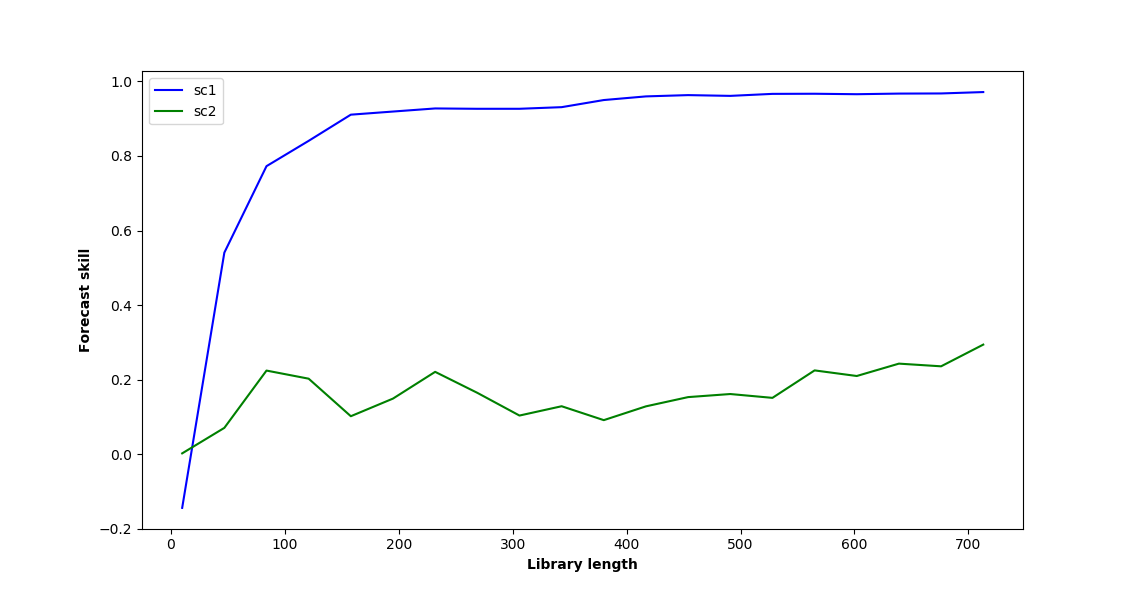
The last graph I obtain where I plot sc1 and sc2 (blue and green curve) differ a little bit from yours. Also, when I change the initial time series parameters to b12=0.2 and b21=0.05, the two curves almost perfectly overlap (which I found surprising since b12 is still 4 times bigger than b21).

See below for the script I used (the main part is code from your tutorial, I just added sections to plot the curves).

Am I missing something?

import numpy as np
import matplotlib.pyplot as plt
import skccm.data as data
import skccm as ccm
from skccm.utilities import train_test_split

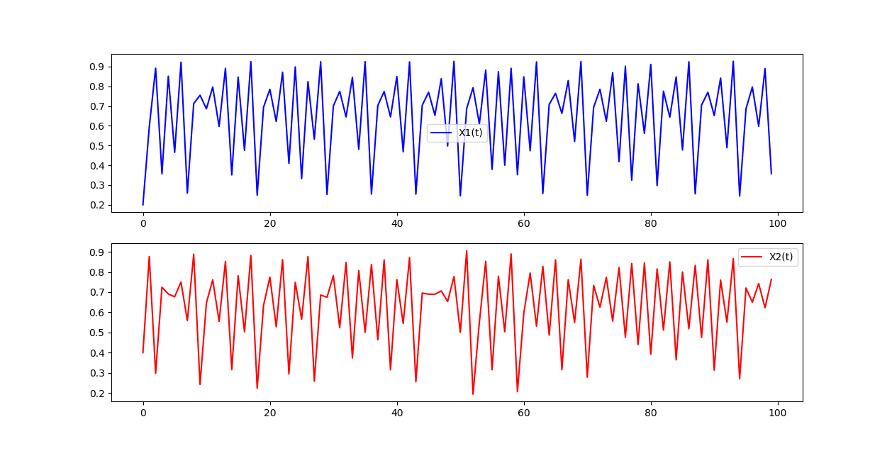
# GRAPH 1
rx1 = 3.72 #determines chaotic behavior of the x1 series
rx2 = 3.72 #determines chaotic behavior of the x2 series
b12 = 0.2 #Influence of x1 on x2
b21 = 0.01 #Influence of x2 on x1
ts_length = 1000
x1,x2 = data.coupled_logistic(rx1,rx2,b12,b21,ts_length)

plt.figure(figsize=(15,8))
plt.subplot(2,1,1)
plt.plot(x1[:100], color='blue', label='X1(t)')
plt.legend(loc='best')
plt.subplot(2,1,2)
plt.plot(x2[:100], color='red', label='X2(t)')
plt.legend(loc='best')
plt.show()

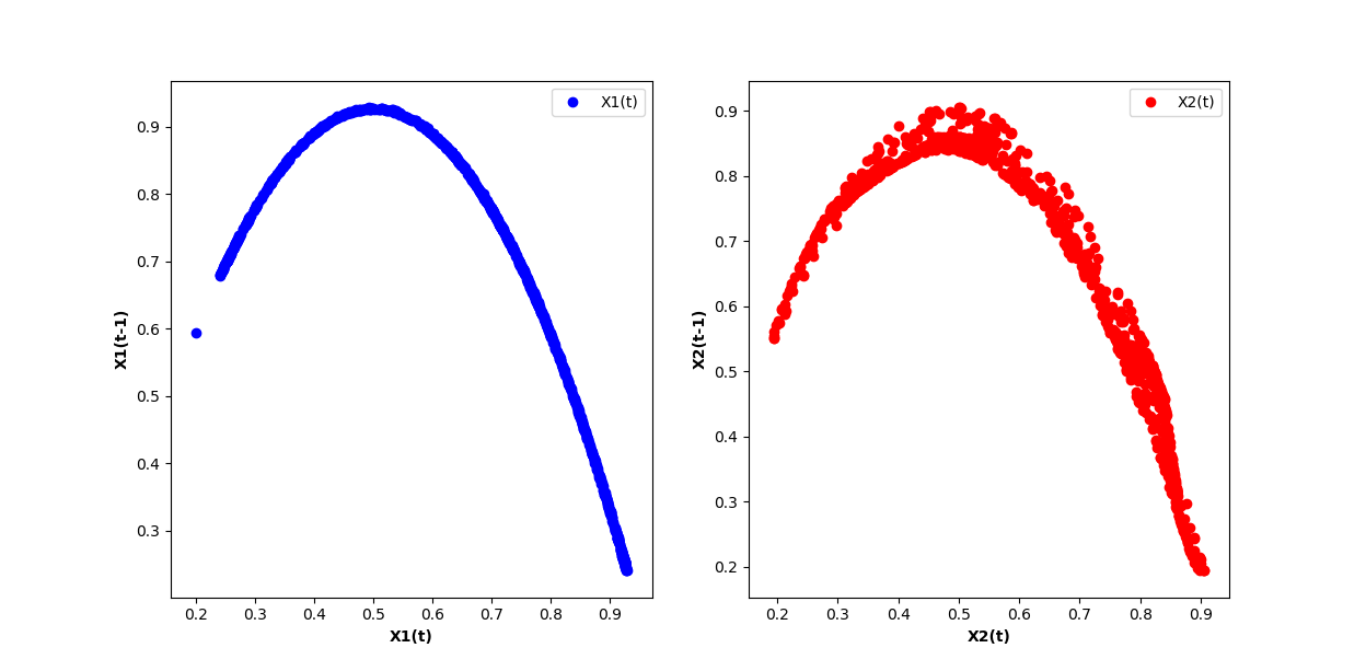
# GRAPH 2
lag = 1
embed = 2
e1 = ccm.Embed(x1)
e2 = ccm.Embed(x2)
X1 = e1.embed_vectors_1d(lag,embed)
X2 = e2.embed_vectors_1d(lag,embed)

plt.figure(figsize=(15,8))
plt.subplot(1,2,1)
plt.scatter(X1[:,0], X1[:,1], color='blue', label='X1(t)')
plt.xlabel('X1(t)', fontweight='bold')
plt.ylabel('X1(t-1)', fontweight='bold')
plt.legend(loc='best')
plt.subplot(1,2,2)
plt.scatter(X2[:,0], X2[:,1], color='red', label='X2(t)')
plt.xlabel('X2(t)', fontweight='bold')
plt.ylabel('X2(t-1)', fontweight='bold')
plt.legend(loc='best')
plt.show()

# GRAPH 3
#split the embedded time series
x1tr, x1te, x2tr, x2te = train_test_split(X1,X2, percent=.75)

CCM = ccm.CCM() #initiate the class

#library lengths to test
len_tr = len(x1tr)
lib_lens = np.arange(10, len_tr, len_tr/20, dtype='int')

#test causation
CCM.fit(x1tr,x2tr)
x1p, x2p = CCM.predict(x1te, x2te,lib_lengths=lib_lens)

sc1,sc2 = CCM.score()

plt.figure(figsize=(15,8))
plt.plot(lib_lens, sc1, color='blue', label='sc1')
plt.plot(lib_lens, sc2, color='green', label='sc2')
plt.xlabel('Library length', fontweight='bold')
plt.ylabel('Forecast skill', fontweight='bold')
plt.legend(loc='best')
plt.show()

[ha0ye]

Hi,

The R version seems to work for b12=0.2 and b21=0.05: CCM rho seems to converge on a higher value in the appropriate direction (from 2 to 1). Does your plot look differently?

library(rEDM)
library(tidyverse)

rx1 = 3.72 #determines chaotic behavior of the x1 series
rx2 = 3.72 #determines chaotic behavior of the x2 series
b12 = 0.2 #Influence of x1 on x2
b21 = 0.05 #Influence of x2 on x1
ts_length = 1000

x1 <- rep(0.2, ts_length)
x2 <- rep(0.4, ts_length)

for(i in seq(ts_length-1))
{
    x1[i+1] = x1[i] * (rx1 - rx1 * x1[i] - b21 * x2[i])
    x2[i+1] = x2[i] * (rx2 - rx2 * x2[i] - b12 * x1[i])
}

df <- cbind(x1, x2)

ccm_12 <- ccm(df, E = 2, lib_sizes = c(10, 20, 40, 80, 160, 400, 800), 
              target_column = 2, lib_column = 1, silent = TRUE)
ccm_21 <- ccm(df, E = 2, lib_sizes = c(10, 20, 40, 80, 160, 400, 800), 
              target_column = 1, lib_column = 2, silent = TRUE)

results <- rbind(ccm_means(ccm_12) %>% mutate(direction = "1 xmap 2"), 
                 ccm_means(ccm_21) %>% mutate(direction = "2 xmap 1"))

ggplot(results, aes(x = lib_size, y = rho, color = direction)) + 
    geom_line() + 
    theme_bw()

Created on 2018-09-24 by the reprex package (v0.2.0).

[julienroyd]

Yes, mine does look different. Here is what I obtain for b12=0.2 and b21=0.05

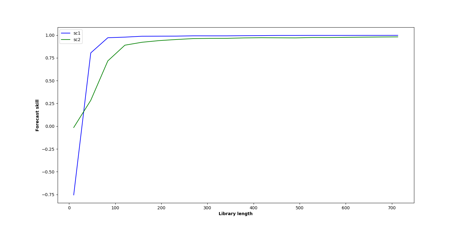
@ha0ye, can you exactly reproduce the results from the Docs using the R version?

[ha0ye]

@julienroy13, using b21 = 0.01, I get something that looks pretty similar to the result in the docs for skccm:

library(rEDM)
library(tidyverse)

rx1 = 3.72 #determines chaotic behavior of the x1 series
rx2 = 3.72 #determines chaotic behavior of the x2 series
b12 = 0.2 #Influence of x1 on x2
b21 = 0.01 #Influence of x2 on x1
ts_length = 1000

x1 <- rep(0.2, ts_length)
x2 <- rep(0.4, ts_length)

for(i in seq(ts_length-1))
{
    x1[i+1] = x1[i] * (rx1 - rx1 * x1[i] - b21 * x2[i])
    x2[i+1] = x2[i] * (rx2 - rx2 * x2[i] - b12 * x1[i])
}

df <- cbind(x1, x2)

ccm_12 <- ccm(df, E = 2, lib_sizes = c(10, 20, 40, 80, 160, 400, 800), 
              target_column = 2, lib_column = 1, silent = TRUE)
ccm_21 <- ccm(df, E = 2, lib_sizes = c(10, 20, 40, 80, 160, 400, 800), 
              target_column = 1, lib_column = 2, silent = TRUE)

results <- rbind(ccm_means(ccm_12) %>% mutate(direction = "1 xmap 2"), 
                 ccm_means(ccm_21) %>% mutate(direction = "2 xmap 1"))

ggplot(results, aes(x = lib_size, y = rho, color = direction)) + 
    geom_line() + 
    theme_bw()

Created on 2018-09-25 by the reprex package (v0.2.0).

[julienroyd]

It is indeed more similar. However it still isn't the same results as in the docs. It seems to me that there might be a reproducibility issue here. @nickc1 have these problems been reported before?

[ha0ye]

Some of it is likely due to random sampling (my default is to use the means over 100 random subsets at each lib_size), among other implementation differences.

[julienroyd]

@ha0ye I'm not sure I understand. How do you set different subsets for each lib_size? Also, I obtain the same results over and over, even when explicitly changing the random seed for numpy and random. Wouldn't that indicate that the differences I get compared to the tutorial aren't due to random sampling?

[ha0ye]

I can only speak for the random implementation for rEDM (the R package version). There, ccm has an argument for the seed (since the RNG is done in underlying C++ and not in R). It might be useful to ping Nick separately via email if he's missing the message here.

[nickc1]

@ha0ye Thanks for helping out and I hope all is well!

@julienroy13 Thanks for the interest and trying out this package. I've been busy the past couple of days, but I will dive into these issues this weekend.

In the meantime, it might be useful to check out some of the example notebooks at: https://github.com/nickc1/skccm/tree/master/scripts

Additionally, this implementation does diverge from the implementation in rEDM. The train-test-split way of creating state spaces is different from the way I believe rEDM does them. This was something I was playing with before I left my research position. I'll have to remind myself of some of the details as I haven't touched this in two years or so, but hopefully I'll have some answers for you soon!

[julienroyd]

Hi @nickc1, Any news regarding this issue?

[nickc1]

Hey @julienroy13,

Spent some time tonight poking around. It looks like the image from the docs was generated with different initial conditions than what the docs show. The docs were also using the same score method as scikit-learn -- https://www.wikiwand.com/en/Coefficient_of_determination. The default method is https://docs.scipy.org/doc/numpy/reference/generated/numpy.corrcoef.html. I'll get that updated. Added an example in the linked notebook below.

The b12=0.2 and b21=0.05 seems to be on the same page with the R version -- same convergence just different axis scales. See the notebook below for a concrete example.

The main difference between the two packages is most likely the random sampling @ha0ye mentioned above - which this package does not implement. Additionally, all of these examples stick to the train-test-split method.

I'll try and find some time to update the docs soon. In the meantime, here is a notebook highlighting the different scoring and some large sample averages.

https://gist.github.com/nickc1/3a1c01a34c97ed5c1021a766c06f7752

Note that I did update the package to allow for the ability to select a scoring method.

https://github.com/nickc1/skccm/commit/81da9a7c1f3d5a1df2ac50d8e1572fb56e8f89dd#diff-e06ea17c08ae1b22e4baa67d6ef4f221

Thanks!