Macrostate or microstate structure and Transition Pathways ?
I was recently trying to analyze a series of MD simulation trajectories using the MSMBuilder and I encountered the following problems:
- how can I obtain the representative structures of the microstates or macrostates of the MSM that I built ?
- I read about the tutorial provided on the official web site of MSMBuilder and the final step produce a trajectory msm-traj.xtc and I wonder whether the frame that I extract from this trajectory can represent the corresponding microstate or macrostate structure ?
- another problem about the msm-traj.xtc trajectory, according to the tutorial, each frame in it corresponds to 1 lag-time unit, so is there a limit for the number of frame of this trajectory, for example, can I generate a msm-traj.xtc trajectory consisting of more than 1000 frames or so ?
- One of the key part of MSM analysis is to find out the transition pathways between various microstates or macrostates. I can find the tpt-related codes such as the path.py but I cannot figure out how to use them and would you please give me a hand ?
Much thanks to your help, thank you!
how can I obtain the representative structures of the microstates or macrostates of the MSM that I built ?
Please take a look at the following ipython notebook which walks through a way to pull micro/macrostate structures from an ensemble of ~20k trajectories.
https://github.com/msmbuilder/paper/blob/master/1-src/ipynbs/src_kinase_msmb_paper_mdl_analysis.ipynb
I read about the tutorial provided on the official web site of MSMBuilder and the final step produce a trajectory msm-traj.xtc and I wonder whether the frame that I extract from this trajectory can represent the corresponding microstate or macrostate structure ?
Yep, the msm-trajectory is a MCMC trajectory going through state space. It is however a randomly picked frame from the microstate, so it might not be representative. However, you can take a look at all the frames assigned to a single state in the msm-traj and that might give you an idea regarding the heterogeneity in the state.
another problem about the msm-traj.xtc trajectory, according to the tutorial, each frame in it corresponds to 1 lag-time unit, so is there a limit for the number of frame of this trajectory, for example, can I generate a msm-traj.xtc trajectory consisting of more than 1000 frames or so ?
There shouldnt be any limit, you can extend them out to 1000 very easily. If you run into any issues there please let us know, thats definitely a bug.
One of the key part of MSM analysis is to find out the transition pathways between various microstates or macrostates. I can find the tpt-related codes such as the path.py but I cannot figure out how to use them and would you please give me a hand ?
Oh, shoot, I cant believe we dont have a tutorial for that. Pinging @brookehus , @jadeshi , @cxhernandez , and other @msmbuilder/developers to see if they have anything lying around .
We don't have any tutorials explicitly written out for TPT (someone should get on that), but here's a notebook for visualizing a path: http://msmbuilder.org/msmexplorer/1.1.0/notebooks/Fs-Peptide.html#Free-Energy-Landscape
Within the msmexplorer.plot_tpaths command, you can see that code for computing the transition pathways is pretty simple:
from msmbuilder import tpt

net_flux = tpt.net_fluxes(sources, sinks, msm)
paths, fluxes = tpt.paths(sources, sinks, net_flux, num_paths=num_paths)
where msm is a MarkovStateModel, sources and sinks are lists of state indices of interest, and num_paths is an optional integer of the number of paths you want to consider.
thanks a lot for your reply and here are the remaining problems:
-
I ran through the code provided on https://github.com/msmbuilder/paper/blob/master/1-src/ipynbs/src_kinase_msmb_paper_mdl_creation.ipynb and https://github.com/msmbuilder/paper/blob/master/1-src/ipynbs/src_kinase_msmb_paper_mdl_analysis.ipynb and I encountered "cmsm_mdl.dict[k]" in the Construct the MSM section (please see In [100], line 4) since I did not find "cmsm" in any other places, I wonder the code here is wrong ? And I try to replace "cmsm" with "msm", which transformed the original code into "msm_mdl.dict[k]", and the overall script can still be carried out and run properly and similar figures and files can be obtained. I am not sure wherther my understanding the "cmsm" issue is correct, and I hope you could please give me a hand and tell me whether it is a mistake or there is a module or function named "cmsm" ?
-
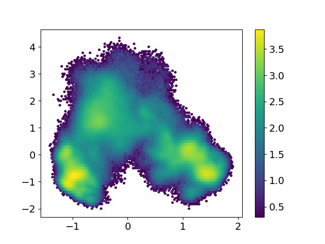
Also regarding the example of src provided on: https://github.com/msmbuilder/paper/blob/master/1-src/ipynbs/src_kinase_msmb_paper_mdl_analysis.ipynb the last section provided by these codes is "Project the model onto dominant slow modes", which seems confusing to me. Since on: https://github.com/msmbuilder/paper/blob/master/1-src/ipynbs/src_kinase_msmb_paper_mdl_creation.ipynb there is already a section called "Plotting the first and second tICS". Both these two sections produce a heatmap/landscape map, I am not quite sure what are the differences between them. Also, I refer to series of papers that also use MSMBuilder to analyze MD simulation trajectories, including the ones from your lab, I find that in most cases, there is only a plot for the first and second tICS instead of a plot of the projection of the model onto the dominant slow modes. So, I wonder these two types of figue or plot, are they the same or at least similar?
-
As for the msm-traj.xtc, I can now understand the lag_time issue and thanks for your explanation. Since you mentioned that this trajectory is a MCMC trajectory so I wonder whetherit can be used for the analysis of the overall process that my simulation want to reproduce ?
-
About the TPT problem, thanks for the information you provided, but I encountered a problem with the version of Python, that is the MSMExplorer you recommended is based on python 3 while my Linux is python 2.7, so I wonder if there is any other possible solution for this mismatch ?
Thank you very much! @msultan @cxhernandez
About the TPT problem, thanks for the information you provided, but I encountered a problem with the version of Python, that is the MSMExplorer you recommended is based on python 3 while my Linux is python 2.7, so I wonder if there is any other possible solution for this mismatch ?
None of the MSMBuilder code provided in my comment above depends on Python 3, nor does the code in tpt.py.
Both these two sections produce a heatmap/landscape map, I am not quite sure what are the differences between them. Also, I refer to series of papers that also use MSMBuilder to analyze MD simulation trajectories, including the ones from your lab, I find that in most cases, there is only a plot for the first and second tICS instead of a plot of the projection of the model onto the dominant slow modes. So, I wonder these two types of figue or plot, are they the same or at least similar?
They are identical.
I hope you could please give me a hand and tell me whether it is a mistake or there is a module or function named "cmsm" ?
Looks like it should be msm_mdl. We can change this in the notebook. @msultan
@cxhernandez I know that your codes are not in python 2, but the module, MSMExplorer, cannot be installed unless it is within a python 3 environment (python 3.5 is needed), which is really troublesome because I think I have to install python 3 and a wide range of other related softwares or modules in order to use the MSMExplorer properly. (btw, using pip to install MSMExplorer has been previously reported as a bug and using conda will lead to the followings: UnsatisfiableError: The following specifications were found to be in conflict:
- msmexplorer -> python 3.5*
- python 2.7* )
@brookehus thanks for your explanation on the tICA and projection onto tICA, but still two little problems remain as follows:
-
For the msm-traj.xtc, according to @msultan this trajectory is a MCMC trajectory, so I wonder whether it can be used for the analysis of the overall process that my simulation want to reproduce ?
-
Within the codes provided on: https://github.com/msmbuilder/paper/blob/master/1-src/ipynbs/src_kinase_msmb_paper_mdl_analysis.ipynb these two lines seem confusing to me:
ind1 = np.where(kmeans_mdl.cluster_centers_[:,0]>1)[0][0] ind2 = np.where(kmeans_mdl.cluster_centers_[:,0]<-0.75)[0][1]
(1) I am not sure how the parameters 1 and -0.75 are chosen, from the heatmap (Out [4]) provided by (In [4]) I guess ? (2) I cannot really figure out the parameter [0][0] or [0][1], how can I find/choose them ? Do I need to refer to the "kmeans_mdl.pkl" (please In [2]) file first?
That's all, thank you very much !
For the msm-traj.xtc, according to @msultan this trajectory is a MCMC trajectory, so I wonder whether it can be used for the analysis of the overall process that my simulation want to reproduce ?
I always use the eigenvectors to interrogate the processes, not a synthetic trajectory. Creating a synthetic trajectory for a longer time than the original simulation will give you more instances of the processes if you want.
I am not sure how the parameters 1 and -0.75 are chosen
We looked at the heatmap and picked them so we could visualize specific microstates where we wanted to.
I cannot really figure out the parameter [0][0] or [0][1], how can I find/choose them ? Do I need to refer to the "kmeans_mdl.pkl" (please In [2]) file first?
Make your own kmeans model and pick indices as appropriate by inspecting the heat map and verifying that the microstates are where you want them. We did this to illustrate the different ends of the energy landscape and used In[150] to pull structures from those microstates. We don't provide the kmeans.pkl file, so yours will be slightly different.
MSMExplorer, cannot be installed unless it is within a python 3 environment (python 3.5 is needed)
Eventually you will need to switch to python 3. numpy is ending support for python 2 in 2019. @cxhernandez can inform more on MSMExplorer, but you can just make a new conda environment with the right version of python instead of changing your main environment.
Eventually you will need to switch to python 3. numpy is ending support for python 2 in 2019. @cxhernandez can inform more on MSMExplorer, but you can just make a new conda environment with the right version of python instead of changing your main environment.
Yep, MSMExplorer is explicitly designed for Python 3.4+ for this reason. As @brookehus mentioned, it's easy enough to create a new environment with Python 3.
My point in referencing MSMExplorer wasn't to recommend using it for this task (in fact, it won't even return the full results of the analysis, so you shouldn't). Just wanted to acknowledge that this is something lacking in the MSMBuilder documentation and point out that the MSMExplorer codebase contains a neat example of how to use the specific MSMBuilder commands that you asked about.
speakinig of the analysis of the heatmap/landscape map produced by two different sections, "Plotting the first and second tICS" and "Project the model onto dominant slow modes", I find my results are a little bit different from the ones provided in the example on:
https://github.com/msmbuilder/paper/blob/master/1-src/ipynbs/src_kinase_msmb_paper_mdl_analysis.ipynb
and
https://github.com/msmbuilder/paper/blob/master/1-src/ipynbs/src_kinase_msmb_paper_mdl_creation.ipynb
the heatmap/landscape maps produced by the two sections in the links above are quite similar and in your previous answers, you said that they are identical.
While in my case, the two heatmap/landscape maps look different
 I believe I carry out the MSM analysis according to the example codes from the two links above, but the corresponding two heatmaps are so different.
I am not sure whether such result is possibly correct or whether I have made any mistake during my analysis.
Many thanks.
@brookehus @msultan
I believe I carry out the MSM analysis according to the example codes from the two links above, but the corresponding two heatmaps are so different.
I am not sure whether such result is possibly correct or whether I have made any mistake during my analysis.
Many thanks.
@brookehus @msultan
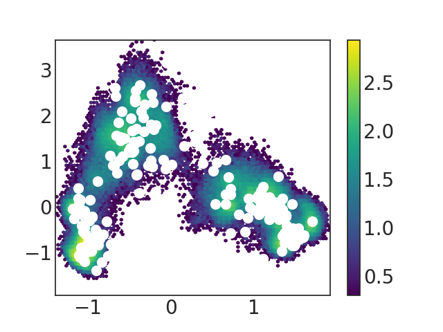
the first figure is produced by "Plotting the first and second tICS" and the second is the result of "Project the model onto dominant slow modes"
That really shouldnt be happening since we dump and then reload the same txx data in the second ipython notebook. Two things come to mind:
1). Did you sub-sample the txx vector? I am guessing it is cutting of the high free-energy regions ( colorbar <0.5) during plotting. trying adding the following arguments
vmin=-1,vmax=4
to the hexbin command.
2). Accidentally over-writing the file. This could happen if you might have been playing with the various parameters and accidentally overwrote the python pickle files.
You can also numerically check that the txx vectors are the same. My guess is that this is just a plotting issue cutting off the high-free energy regions.
i think i have sub-sample the txx vector in the section called "Subsample the data for faster processing" on https://github.com/msmbuilder/paper/blob/master/1-src/ipynbs/src_kinase_msmb_paper_mdl_analysis.ipynb
and i changed my code according to your suggestions but still, the output is similar. here is my edited code:
#load the necessary models tica_mdl = verboseload("tica_mdl.pkl") tica_data=dataset("./reg_ticas_500lt_10tics/")
kmeans_mdl = verboseload("kmeans_mdl.pkl")
msm_mdl = ContinuousTimeMSM() msm_mdl.dict.update(**pickle.load(open("msm_mdl.pkl",'rb')))
sub_tica_data = [tica_data[i] for i in np.arange(0,len(tica_data),10)] ktree=KDTree(sub_tica_data) txx=np.concatenate(sub_tica_data) sl=list(msm_mdl.mapping_.keys())
sns.set_style('white') p=matplotlib.pyplot.hexbin(txx[:,0],txx[:,1],bins='log',mincnt=1,cmap='viridis',vmin=-1,vmax=4) matplotlib.pyplot.scatter(kmeans_mdl.cluster_centers_[sl,0],kmeans_mdl.cluster_centers_[sl,1],s=100,c='white') matplotlib.pyplot.colorbar(p)
matplotlib.pyplot.savefig('project-1_0409.png')
ind1 = np.where(kmeans_mdl.cluster_centers_[:,0]>0.55) [0][60]
matplotlib.pyplot.figure(figsize=(12,8)) sns.set_style('white') p=matplotlib.pyplot.hexbin(txx[:,0],txx[:,1],bins='log',mincnt=1,cmap='viridis',vmin=-1,vmax=4) matplotlib.pyplot.scatter(kmeans_mdl.cluster_centers_[ind1,0],kmeans_mdl.cluster_centers_[ind1,1],s=300,c='black',marker='*')
matplotlib.pyplot.xlabel("Projection On 1st Tic",size=22) matplotlib.pyplot.ylabel("Projection On 2nd Tic", size=22) cb=matplotlib.pyplot.colorbar(p) cb.set_label(size=22,label="Log Count")
matplotlib.pyplot.savefig('project-2_15_0409.png')
and the figure i get:
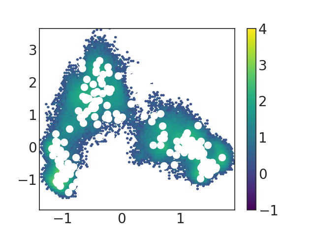
it seems that the heatmap hasn't changed much?
thanks.
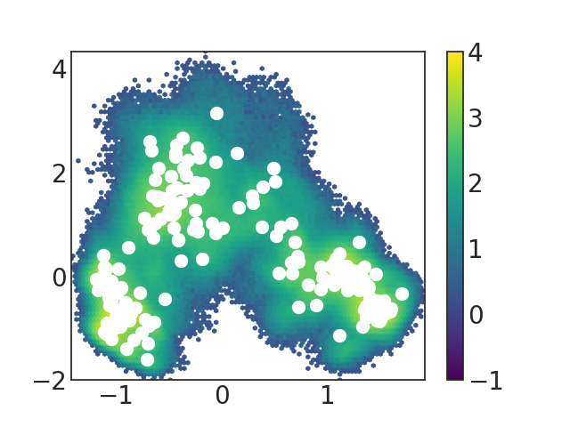
i try to delete the "Subsample the data for faster processing" section code and change my code into the following:
``ktree=KDTree(tica_data) txx=np.concatenate(tica_data) sl=list(msm_mdl.mapping_.keys())
sns.set_style('white') p=matplotlib.pyplot.hexbin(txx[:,0],txx[:,1],bins='log',mincnt=1,cmap='viridis',vmin=-1,vmax=4) matplotlib.pyplot.scatter(kmeans_mdl.cluster_centers_[sl,0],kmeans_mdl.cluster_centers_[sl,1],s=100,c='white') matplotlib.pyplot.colorbar(p)
matplotlib.pyplot.savefig('project-1_0409_2.png')
ind1 = np.where(kmeans_mdl.cluster_centers_[:,0]>0.55) [0][60] #IF [:,0}] FIRST [] CAN NOT BE 1 "TUPLE INDEX OUT OF RANGE"
matplotlib.pyplot.figure(figsize=(12,8)) sns.set_style('white') p=matplotlib.pyplot.hexbin(txx[:,0],txx[:,1],bins='log',mincnt=1,cmap='viridis',vmin=-1,vmax=4) matplotlib.pyplot.scatter(kmeans_mdl.cluster_centers_[ind1,0],kmeans_mdl.cluster_centers_[ind1,1],s=300,c='black',marker='*')
matplotlib.pyplot.xlabel("Projection On 1st Tic",size=22) matplotlib.pyplot.ylabel("Projection On 2nd Tic", size=22) cb=matplotlib.pyplot.colorbar(p) cb.set_label(size=22,label="Log Count")
matplotlib.pyplot.savefig('project-2_15_0409_2.png')
and it seems that the problem can be solved and the figure i get is as below:
previously, @brookehus talked about analyze the trajectories produced based on MSM analysis and she said she recommended using eigenvectors for analysis rather than the synthetic trajectory. In the tutorial on http://msmbuilder.org/3.8.0/tutorial.html I found two kinds of trajectories are produced:
- using the tica-sample-coordinate,py, which gives tica-dimension-o.xtc
- using the microstate-traj.py, which gives msm-traj.xtc
I wonder whether the first one is the eigenvector that brookehus has talked about ? Also, in the paper by your lab entitled "Activation pathway of Src kinase reveals intermediate states as targets for drug design", MSM trajectories calculated using a Monte Carlo algorithm are used for analysis. So I think both of these two kinds of trajectories produced along the MSM analysis process can be used for further analysis ? Thanks.
My two cents: the first trajectory is used to interpret what molecular 'movement' the first tIC is capturing. For the tutorial example, this corresponds to the 'folding' of the peptide. In my experience, in more complex situations this is not as interpretable as it gives a really 'jumpy' trajectory, where many degrees of freedom are changing at the same time, so it can be quite confusing. The devs can correct me if I'm wrong but there is no 'time' in this trajectory, the frames are sampled from the tIC projection.
The second trajectory is trying to visualize what a long trajectory would look like, by generating a set of microstate jumps from the transition matrix that you have estimated. In my opinion, this is interesting because it gives you a visual intuition of how long it actually takes to go from one part of your phase space to the other. But it really doesn't add anything to the analysis since you're only going to see whatever is encoded by the transition matrix you've estimated. In this trajectory, each frame is separated by whatever time unit you chose to build your MSM with. So for example, if you're loading all the frames in your trajectories, and each frame is separated by 200 ps, and then you build an MSM with a lag time of 10, that is a lag time of 2 ns. So each frame in your 'synthetic' trajectory will be spaced by 2 ns.
if so, what trajectory or data should I use to analyze properties such as RMSD of the overall process that the MSM covers ? The only way I can think about is to use the trajectory correspond to the MSM. Thanks,
also, when I try with the microstate-traj.py script, in the tutorial, the overall process uses a DihedralFeaturizer and in my own case, I use a AlphaAngleFeaturizer. Then, it comes to an error as follows:
Traceback (most recent call last):
File "microstate-traj.py", line 23, in
my code for microstate-traj.py are as below: """Sample a trajectory from microstate MSM
msmbuilder autogenerated template version 2 created 2018-03-05T17:35:31.310126 please cite msmbuilder in any publications
"""
import mdtraj as md
from msmbuilder.io import load_trajs, save_generic, preload_top, backup, load_generic from msmbuilder.io.sampling import sample_msm
meta, ttrajs = load_trajs('ttrajs') msm = load_generic('msm.pickl') kmeans = load_generic('kmeans.pickl')
inds = sample_msm(ttrajs, kmeans.cluster_centers_, msm, n_steps=2000, stride=1) save_generic(inds, "msm-traj-inds.pickl")
top = preload_top(meta) traj = md.join( md.load_frame(meta.loc[traj_i]['traj_fn'], index=frame_i, top=top) for traj_i, frame_i in inds )
traj_fn = "msm-traj.mdcrd" backup(traj_fn) traj.save(traj_fn)
I am not sure whether it is because I changed the featurizer for the whole process in the very beginning or anything else? And I can I tackle it?
Many thanks for your help.
i don't think it is a problem to do with the featurizer because when I try with the original featurizer used in the tutorial, that is the DihedralFeaturizer, the same problem also occurs as follows:
[customer@node01 msm]$ python microstate-traj.py
/home/customer/anaconda2/lib/python2.7/site-packages/sklearn/cross_validation.py:41: DeprecationWarning: This module was deprecated in version 0.18 in favor of the model_selection module into which all the refactored classes and functions are moved. Also note that the interface of the new CV iterators are different from that of this module. This module will be removed in 0.20.
"This module will be removed in 0.20.", DeprecationWarning)
/home/customer/anaconda2/lib/python2.7/site-packages/sklearn/grid_search.py:42: DeprecationWarning: This module was deprecated in version 0.18 in favor of the model_selection module into which all the refactored classes and functions are moved. This module will be removed in 0.20.
DeprecationWarning)
/home/customer/anaconda2/lib/python2.7/site-packages/statsmodels/compat/pandas.py:56: FutureWarning: The pandas.core.datetools module is deprecated and will be removed in a future version. Please use the pandas.tseries module instead.
from pandas.core import datetools
Traceback (most recent call last):
File "microstate-traj.py", line 23, in
I have no idea where to start debugging for such error.
Thanks.
i think your ttrajs is not the right shape. ttrajsshould be of the shape N,T where N is the number of frames and T is number of tICs. Could you start an interactive ipython notebook and try the following code.
import mdtraj as md

from msmbuilder.io import load_trajs, save_generic, preload_top, backup, load_generic
from msmbuilder.io.sampling import sample_msm

meta, ttrajs = load_trajs('ttrajs')

print(ttrajs)
print(ttrajs.shape)
The other thing that might be an issue, though is unlikely, is that this is a weird python2 vs python 3 issue. When @mpharrigan wrote the io module, he was already on python 3.
Also thank you @jeiros , I wouldn't have been able to explain it better myself. You are right, the tICA-trajectories have no time information, they are designed to simply try to understand what the tICs represent. It equal to linearly sampling along any reaction coordinate/CV so it integrates out all other CVs which makes the movies "jumpy" . For any observable (such as RMSD etc) based analysis, we recommend using the long MSM trajectories.
As for the trajectories based on MSM I wonder what's the time order for them? Since I notice that some structure snapshots reappear for many times throughout the MSM trajectories and it seems that for a specific microstate within the trajectory, it will be visited several times seperately. Also to mention is the Nature Communication paper on Src kinase, it seems that the MSM trajectory there goes through transition between active and inactive states several times, which seems strange to me because I guess the MSM for the activation pathway of kinase should only be the transition between inactive and active for only one time? Thank you very much.
As for the trajectories based on MSM I wonder what's the time order for them?
The time between frames is the MSM lagtime.
Since I notice that some structure snapshots reappear for many times throughout the MSM trajectories and it seems that for a specific microstate within the trajectory, it will be visited several times seperately.
Yea, its possible if you only have a few frames in a state that they get picked multiple times as you go in and out of that microstate.
Also to mention is the Nature Communication paper on Src kinase, it seems that the MSM trajectory there goes through transition between active and inactive states several times, which seems strange to me because I guess the MSM for the activation pathway of kinase should only be the transition between inactive and active for only one time?
The MSM is a model of the underlying process. We can go between them using these synthetic trajectories as many times as we want. For example, consider a process A <-> B <->C. What the MSM does is model the entire process using trajectories that go from A->B, B->C, C->B,C->A ... Then once we have the model built, we can now go from A-> B->C->B->A as many times as we want because we understand what the transition probabilities and timescales of going between these metastable states are.
first, if the time between each frame is the MSM lagtime, then if I set the number of frames to be extremely high, the length of the synthetic trajectory will far exceed the length of the MSM or the total MD trajectories that I use to construct MSM, which seems weird ? Also, it seems to me that the length of the MSM synthetic trajectory is related to how many times that different intermediate state convert into each other?
as for the reappearance of the same structure snapshot, I mean sometime during the synthetic trajectory, the structure just keep unchanged for a certain time, I am not sure whether it is wrong with my choice of the length of synthetic trajectory or anything else. Thanks.
The structure not changing for several frames should be pretty normal, because in general the self-transition probability of a state is much larger than interstate transition probabilities. This is actually one of the properties you want to see when you build a MSM, since that means the protein has time to randomly wiggle around in its current state and "forget" where it came from before going somewhere else, i.e. the definition of Markovian. Your synthetic MSM trajectory is just sampling from your transition matrix, so it's not uncommon for the protein to just stay in the same state for a long time.
As for your other question regarding running the MSM trajectory longer than the original simulation, that's perfectly fine, because you're not actually generating any new information from the MSM trajectory, just reproducing known data. If you run a microsecond of MD and create a millisecond MSM trajectory, the MSM is not actually running new simulations and exploring new parts of the free energy landscape for you. It's just repeating what you've seen in your original MD simulation over and over again.
As a stupid example, if you have a protein that folds on the millisecond timescale and you run a microsecond of MD, creating a MSM trajectory a millisecond long will not magically fold the protein for you, since you haven't actually sampled those dynamics in the actual MD data.