Geom/stat for uncertainty in stacked / cumulative proportions

[mjskay]

Maybe something for bars and/or areas. See this twitter thread w/ @ASKurz @bwiernik on bars and things: https://twitter.com/SolomonKurz/status/1372632774285348864?s=20 ... which might be doable using a stat combined with geom_slabinterval.

And this from @tjmahr on areas: https://twitter.com/tjmahr/status/1456278108311625728?s=20 ... which is more difficult. The ideal version might be a gradient approach, maybe something backed by geom_raster. That or think if there's a lineribbon generalization for this... (maybe the trick is an analog to median_qi for cumulative probabilities with one-sided intervals?)

[mjskay]

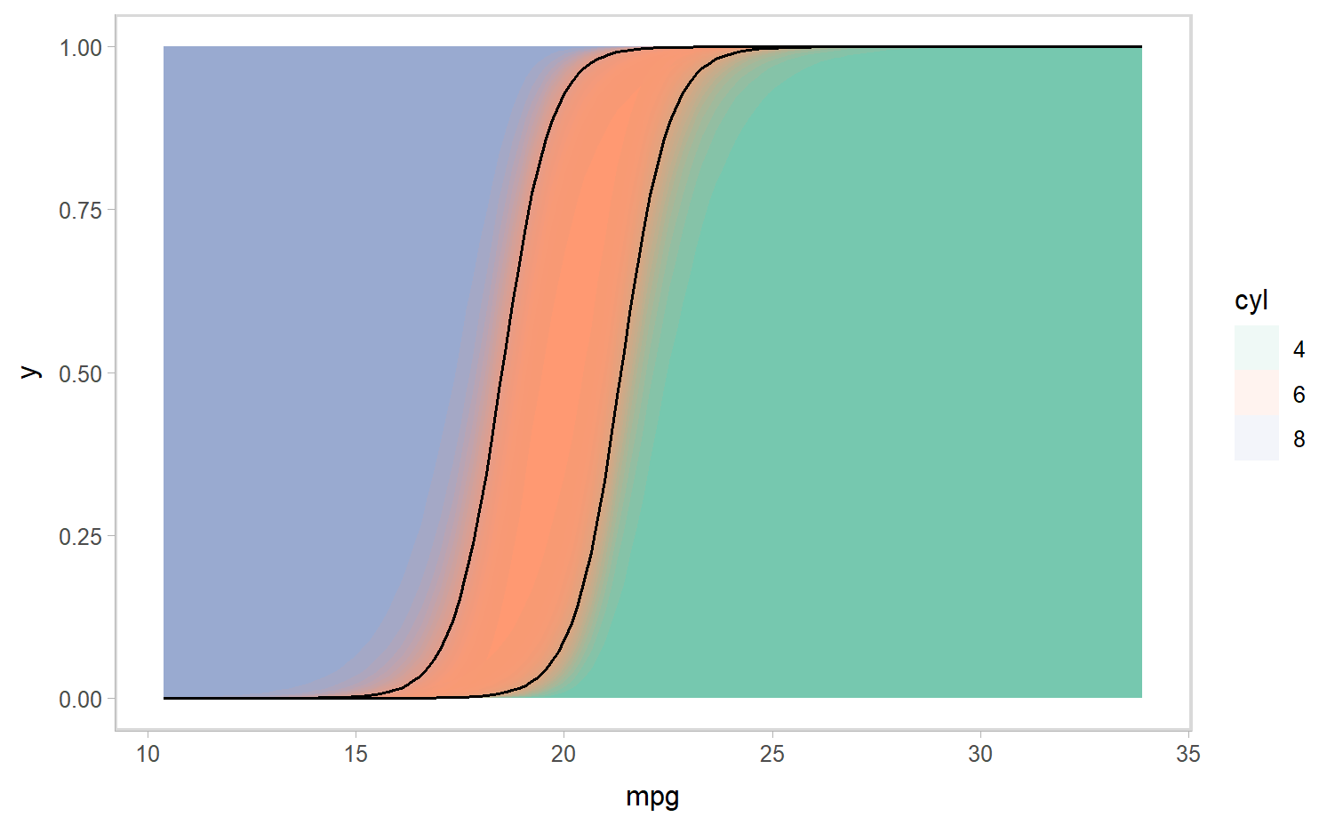
Okay I hacked something together for the continuous case based on the example in the tidy-brms vignette:

probs = ppoints(21)

mtcars_clean %>%
  data_grid(mpg = seq_range(mpg, n = 150)) %>%
  add_epred_draws(m_cyl, value = "P(cyl == c | mpg)", category = "cyl") %>%
  arrange(cyl) %>%
  group_by(.draw, .row, mpg) %>%
  mutate(
    `P(cyl <= c | mpg)` = cumsum(`P(cyl == c | mpg)`),
    `P(cyl < c | mpg)` = `P(cyl <= c | mpg)` - `P(cyl == c | mpg)`
  ) %>%
  group_by(cyl, mpg, .row) %>%
  summarise(
    across(c(`P(cyl <= c | mpg)`, `P(cyl < c | mpg)`), quantile, probs = probs),
    .prob = probs,
    .groups = "drop_last"
  ) %>%
  ggplot(aes(x = mpg, ymin = `P(cyl < c | mpg)`, ymax = `P(cyl <= c | mpg)`)) +
  geom_lineribbon(aes(fill = cyl, group = interaction(.prob, cyl), y= 0), alpha = .1, color = NA) +
  # using ribbon instead of lineribbon will "work" (in the sense a plot is drawn)
  # but because of the draw order of the ribbons is biased towards higher values of
  # cyl so the gradients don't appear centered on the median; geom_lineribbon
  # addresses this by interleaving the ribbons
  # geom_ribbon(aes(fill = cyl, group = interaction(.prob, cyl), y= 0), alpha = .1, color = NA) +
  geom_line(aes(group = cyl, y = `P(cyl <= c | mpg)`), data = . %>% filter(.prob == 0.5, cyl != levels(cyl)[nlevels(cyl)])) +
  scale_fill_brewer(palette = "Set2")

Simple next step would be to add this to that vignette. Possibly more useful would be to think about the categorical case, mock that up, then try to generalize something useful for both cases (which might be an analog to point_interval for cumulative data and/or stats to go with this).

[ASKurz]

I wonder if this or something similar could be applied to nominal models. Consider my facetted plot at the end of Section 22.3.3.1, which is based on a brms model for which family = categorical(link = logit). For that visualization, I just used the posterior means for the background fill. It would be great if there was a principled way to insert uncertainty.

[mjskay]

Yeah I think this could also be used for nominal models. That faceted plot (and the Twitter conversation that led to it) was part of the impetus for this issue 🙂

[ASKurz]

Then you've got one hot vignette in the works. I'll probably end up revising some of my Chapter 22 to showcase your efforts.