webgpgpu

This library contains a series of walk-through examples, starting from "hello GPU" and slowly building up to simulating spatiotempoal PDEs/IDEs (e.g. pnmeila, woitzel, houston, inear).

The aim is to construct minimal examples using only HTML, Javascript and WebGL (no libraries).

Previews and descriptions of the examples can be found here, and the files contained in this repository can be browsed on Github pages.

Explore project contents in browser: examples and (not quite) games.

Other examples of using WebGL for GPGPU code can be found here (1 2 3 4 5).

Basic examples

Basic examples that set up a two-dimensional rendering environment within the 3D WebGL framework, and then illustrate basic rendering techniques like rendering from a texture, pixel operations like blurring, and random noise.

	Example 1: "Hello GPU" (run in browser) Set up an HTML Canvas for webGLM rendering, and render a simple coordinate-dependent image.
	Example 2: "1D texture" (run in browser) Use a one-dimensional texture as a colormap. Eventually, we will also render to texture to store rendering and simulation data between frames.
	Example 3: "Use two textures" (run in browser) Basic example loading two different colormaps as textures. Using multiple textures is important for rendering more complex systems, which may require more state than a single red-green-blue texture can store.
	Example 4: "Pixel blur" (run in browser) Simple vertical blur by averaging nearyby pixel values. an image.
	Example 5: "Separable Gaussian blur" (run in browser) We can compute larger Gaussian blurs quickly by blurring first horizontally and vertically.
	Example 6: "Multi-color blur" (run in browser) For simulations, different colors might represent different quantities. This Gaussian blur kernel treats each color channel separately, blurring them by different amounts.
	Example 7: "Noise" (run in browser) Stochastic simulations and animations require a source of noise. This kernel approximates uniform pseudorandom number generation, in a fast ad-hoc way that is suitable for visualizations (not not guaranteed to be random enough for other uses).
	Example 8: "Spatiotemporal noise" (run in browser) This example combines driving noise with repeated Gaussian blurs to create a spatiotemporal noise effect.
	Example 11: "Bitops" (run in browser) The minimal subset of WebGL doesn't explicitly support storing/reading unsigned integer types from textures, or bit operations. However, most reasonable hardware and WebGL implementations should implicitly store color texture data as 8-bit integers. This kernel accesses this color data as if it were uint8, even though it is technically a float.

Image processing examples

These examples demonstrate basic image processing: color adjustments and blur/sharpen.

	Example 15: "Load image" (run in browser) This example loads an image resource, copies it to a texture, and displays it on screen.
	Example 16: "Linear hue rotation" (run in browser) This example demonstrates hue rotation as an optimize linear transformation using hue and chroma.
	Example 17: "Image blur" (run in browser) Apply iterated Guassian blur to image data.
	Example 17b: "Unsharp mask" (run in browser) Apply iterated unsharp mask to image data.
	Example 19: "Brightness and contrast" (run in browser) Adjust brightness and contrast of image based on mouse location.
	Example 19: "Hue and saturation" (run in browser) Adjust hue and saturation of image based on mouse location.

Technical experiments

These examples test a couple of technical tricks that might be useful in rendering.

	Example 25: "Gaussian noise" (run in browser) Convert uniform random numbers to Gaussian random numbers with mean and variance specified by the mouse location.
	Example 21: "Recursive mipmaps" (run in browser) Mipmaps are successively downsampled copies of a texture that are used to avoid aliasing. The are usually computed once, with a program is initialized. However, if we are rendering to texture data, and then want to use that data as a texture to color 3D objected, we may want to updates mipmaps. Rather than update all texture resolutions at once, however, we successively downsample on each iteration. meaning that lower-resolution mipmaps are updated later.
	Example 25: "Statistical mipmaps" (run in browser) Texture mipmaps compute the average texture color over a region, by downsampling. What if we'd like the average statistics, like mean and variance, over a given region?
	Example 25: "Hello particles" (run in browser) Particle systems are useful in many-body simulations. This example uses texture data for particle location, and also renders each particle differently based on an offset into a texture.
	Example 13: "Julia set" (run in browser) Track the mouse location and render a Julia set using video feedback.

Psychedelic

These examples are "Just for fun"

	Example 9: "Quadratic feedback" (run in browser) Quadratic video feedback example of iterated conformal maps which can be used to render Julia set fractals.
	Example 10: "Logarithmic feedback" (run in browser) Iterated logarithmic video feedback. The logarithmic map can be used to approximate the coordinate mapping from visual cortex to retinal (or "subjective") coordinates, which explains why some visual hallucinations take on a tunnel appearance. (Ermentrout GB, Cowan JD. A mathematical theory of visual hallucination patterns. Biological cybernetics. 1979 Oct 1;34(3):137-50.)
	Example 18: "Psychedelic filter" (run in browser) Applies a combination of blues, sharpening, and hue rotations for a psychedelic image effect.
	Example 14: "Complex arithmetic" (run in browser) Interpret length-2 vectors as complex numbers using a collection of macros. More sophisticated video feedback example.
	Example 17: "Quasicrystal 1" (run in browser) An infinitely-zooming quasicrystal visualization with Shepard tone accompaniment, black and white.
	Example 17: "Quasicrystal 2" (run in browser) An infinitely-zooming quasicrystal visualization with Shepard tone accompaniment, color.

Neural field simulations

Using only 8-bit color data to store state values means that these neural field simulations are only approximate. Some dynamical behaviors won't appear at parameters quite qhere the theory predicts. However, most qualitative behaviors are preserved.

	Example 1: "Wilson-Cowan equations" (run in browser) Spiral wave emerge in a Wilson-Cowan neural field model. The lack of platform-specified rounding in WebGL means that these patteerns to not appear correcrtly on all devices (see example 2).
	Example 2: "Platform independent rounding" (run in browser) Spiral wave emerge in a Wilson-Cowan neural field model. Additional macros enforce a platform-independent rounding rule, allowing for consistent behavior across devices.
	Example 3: "Center-surround" (run in browser) Center surround "mexican hat" style coupling leads to the emergence of striped patterns in a Wilson-Cowan system.
	Example 4: "Flicker" (run in browser) Turing patterns induced in a Wilson-Cowan system by periodic forcing. (Rule M, Stoffregen M, Ermentrout B. A model for the origin and properties of flicker-induced geometric phosphenes. PLoS computational biology. 2011 Sep 29;7(9):e1002158.)
	Example 5: "Retinotopic map" (run in browser) Use the logarithmic map to approximate how a Wilson-Cowan pattern forming system might appear in subjective coordinates, if the emergent waves were to occur in visual cortex. (Ermentrout GB, Cowan JD. A mathematical theory of visual hallucination patterns. Biological cybernetics. 1979 Oct 1;34(3):137-50.)
	Example 9: "16-bit precision" (run in browser) Use two color components, with 8-bits each, to implement 16-bit fixed-point storage of simulation states. This leads to a slightly more accurate numerical integration.
	Example 10: "Fullscreen" (run in browser) Full-screen test of a logarithmically-mapped Wilson-Cowan pattern forming system.
	Example 11: "Psychedelic" (run in browser) Full-screen test of a logarithmically-mapped Wilson-Cowan pattern forming system. Additional noise and hue rotation effects are added. This is purely a visual demonstration.

"Games"

Not actually games, but rather explorations of using a tile shader with various cellular automata. The first few examples just set up basic (1) html, render a (2) test canvas, and then check that things are (3) working with the webgpgpu javascript library. The next few examples check that we've configured the (4) viewport correctly, and build up (5) mouse and (6) keyboard interaction. The remaining examples render fun things like...

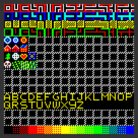	Game Example 7: "Hello Texture" (run in browser) Load a texture of 256 8×8 tiles from a web resource. We'll use this texture to render pixels of the game not as colors, but as character-like tiles. Mouse and keyboard zoom/pan should work.
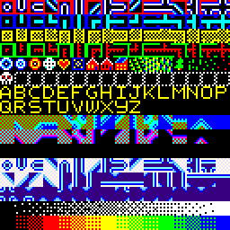	Game Example 8: "Base64 Texture" (run in browser) Encode texture in javascript source in base64. This side-steps the cross-domain restrictions and makes it slightly less painful to edit the texture locally when developing. Mouse panning and zoom should work.
	Game Example 9: "Hello Tiles" (run in browser) Get a tile shader working that renders 8x8 tiles at a large size to the screen, with 1:1 matching of canvas to device pixels.
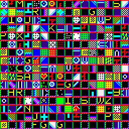
	Game Example 10: "Hello Noise" (run in browser) Tests random number generation and renders noisy pixels as randomly selected tiles from a texture of 256 8x8 pixel tiles.
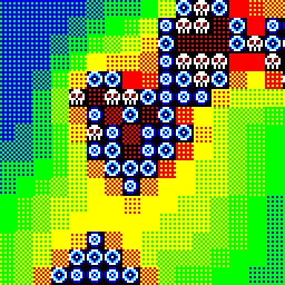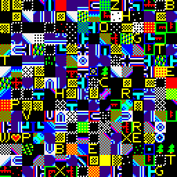
	Game Example 11: "Game of Life" (run in browser; large; small for mobile) Conway's game-of-life with a wacky tile shader. Dying cells are skulls. Colors diffuse outward from living areas.
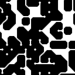
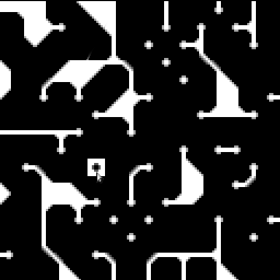
	Game Example 12: "Dendrites" (run in browser) Cellular automata performing a sort of diffusion-limited aggregation. Dendrites grow from seed points, avoiding self-intersection. Refresh the page to get one of four tile sets at random.
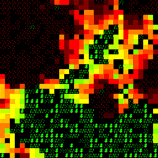	Game Example 13: "Forest Fire" (run in browser; large) Forest fire cellular automata. Trees burn, turn to ash, then grass, then shrub, then trees, then burn again. Should be close-ish to criticality, and generate patterns at a range of scales. Same as the model for developmental retinal waves in this paper.
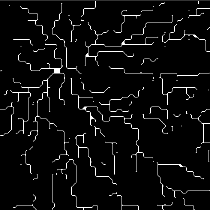
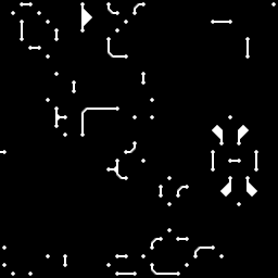
	Game Example 12 variant: "Neural Dendrites" (run in browser) Nucleate invisible dendrites from a seed. Around the environment are scattered invisible targets ("synapses"). When a dendrite forms a synapse, it becomes visible. Store a distance-from-seed value in the invisible exploratory dendrite in order to trace a path back to the seed ("cell").
	Game Example 14: "Marching Squares" (run in browser) Broken/ugly terrain example with marching squares.
	Game Example 15: "Marching Squares" (run in browser) Terrain example with marching squares, less broken.
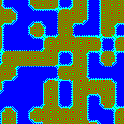
	Game Example 17: "Marching Boxes" (run in browser) Marching boxes shader as described in this post.
	Game Example 17b: "Marching-Boxes Game of Life" (run in browser) Conways game of life rendered with the marching boxes shader.
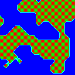
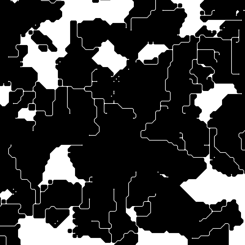
	Game Example 17c: "Map Generator" (run in browser) Generates terrain using a diffusion-smoothed noise-driven height field. Thresholds tis to demarcate land/boundary. Runs a variant of the dendrites cellular automata to add rivers.
	Game Example 18: "Read/write data in texture" (run in browser) Explores several methods of modifying texture data. Test A calls an entire shader to read/edit/write a single pixel; surprisingly faster than reading data back of the GPU (Test B, C). Don't do use either method! Test D prints benchmarks to the console (run it). On my system, using a shader with full viewport costs 42 ms; Restricting viewport to single pixel took longer, 131 ms. Reading-writing using memory copy took a whopping 1.3 s. Simply setting a pixel took 11 ms. TLDR: the best method is to retain a copy of the game state on the CPU. Do any editing there, then transfer the changes write-only with a memory copy to the GPU.
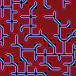
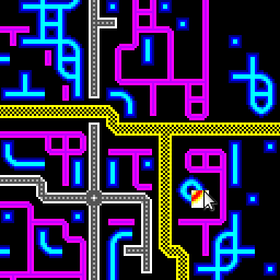
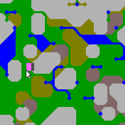
	Game Example 18: Draw Pipes (run in browser) Mouse interaction lets you edit a map to draw draw roads, pipes, cables. Inspired by classic sim city.
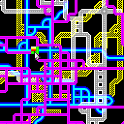
	Game Example 20: "Layered Pipe-Drawing Kernel" (run in browser) Same as example 19, but now we composite layers atop one another, so pipes/roads/cabels can cross. Still stores all the game state in the RGBA color data of a texture.
	Game Example 21: Layered Terrain Edit (run in browser) This is unfinished. Goal was to make a map editor with different elevations of terrain, rendered using the "marching boxes" shader.

Unless otherwise specified, media, text, and rendered outputs are licensed under the Creative Commons Attribution Share Alike 4.0 license (CC BY-SA 4.0). Source code is licensed under the GNU General Public License version 3.0 (GPLv3). The CC BY-SA 4.0 is one-way compatible with the GPLv3 license.