Inverse Transform + Transform does not produce correct points

[fshriver]

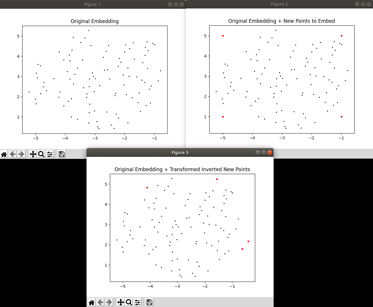
I noticed that when using inverse_transform(), points in the high-dimensional space that are inverted from points in the low-dimensional space do not go back to their expected positions in the low-dimensional space when run through transform() again. I've provided a very simple script below, where I generate some fake data and made an embedding out of it, then I create some arbitrary points which lie within the embedding. I then invert those arbitrary points to what they would look like in the high-dimensional space and then immediately transform them back using the same fitted UMAP model I just used. I've attached a screenshot of the result I see on my end: as you can see, the arbitrary points in red do NOT return to their initial set positions. You can uncomment the plt.show() at the end of the file if you want to see the plots for yourself.

I'm not sure if I'm using inverse_transform() wrong or if there's a bug in the function? The only thing of note that I'm doing is that I'm setting random_state, but it doesn't seem intuitive that that would affect the inverse transform. This may also be connected to https://github.com/lmcinnes/umap/issues/515.

import numpy as np
import matplotlib.pyplot as plt
import umap

# Set random seed so you can see the exact same data I do
np.random.seed(42)

# Generate random data for initial embedding
original_data = np.random.random(size = (100,50))

# Transform and plot embedding
transformer = umap.UMAP(n_neighbors=10, min_dist=0.1, random_state=42).fit(original_data)
original_embeddings = transformer.transform(original_data)
plt.figure()
plt.scatter(original_embeddings[:,0], original_embeddings[:,1], s=2, c = 'black')
plt.title('Original Embedding')

# Create a few new points in the embedding that we'll want to invert, and plot them
new_embeddings = np.zeros(shape = (4,2))
new_embeddings[0,0] = -5
new_embeddings[0,1] = 1
new_embeddings[1,0] = -1
new_embeddings[1,1] = 1
new_embeddings[2,0] = -5
new_embeddings[2,1] = 5
new_embeddings[3,0] = -1
new_embeddings[3,1] = 5
plt.figure()
plt.scatter(original_embeddings[:,0], original_embeddings[:,1], s=2, c = 'black')
plt.scatter(new_embeddings[:,0], new_embeddings[:,1], s=10, c = 'red')
plt.title('Original Embedding + New Points to Embed')

# Invert new points and then transform them using the same parent they were just inverted from
inv_new_embeddings = transformer.inverse_transform(new_embeddings)
transformed_inv_new_embeddings = transformer.transform(inv_new_embeddings)
plt.figure()
plt.scatter(original_embeddings[:,0], original_embeddings[:,1], s=2, c = 'black')
plt.scatter(transformed_inv_new_embeddings[:,0], transformed_inv_new_embeddings[:,1], s=10, c = 'red')
plt.title('Original Embedding + Transformed Inverted New Points')

# Uncomment me if you want to see plots
plt.show()

[lmcinnes]

Both the inverse transform and transform are stochastic approximations, so there is going to be some noise involved in this. Unfortunately this means that round-tripping like this is unlikely to land you back in exactly the same spot. The more data you have the less things will move on a qualitative level, but you will still see variation.

[mxposed]

@lmcinnes I was just trying the inverse_transform method and found out that I cannot reconstruct my original 30-dimensional points which I just embedded on 2d back. Is this expected? Even with the fixed random seed? How small/large should the error be?

[lmcinnes]

Both directions are stochastic. Fixing a random seed will merely make the same stochastic errors occur each time you do it. Exactly how big the error will be will depend on the dataset (and whether your particular points are in dense or sparse regions; the sparser the region, the bigger the round trip error will tend to be). Usually it should be fairly close, but note that close is with respect to the rest of the dataset; ideally it will be more like the original than other further away data samples.