[Not for Merge]: Visualize the gradient of each node in the lattice.

[csukuangfj]

This PR visualizes the gradient of each node in the lattice, which is used to compute the transducer loss.

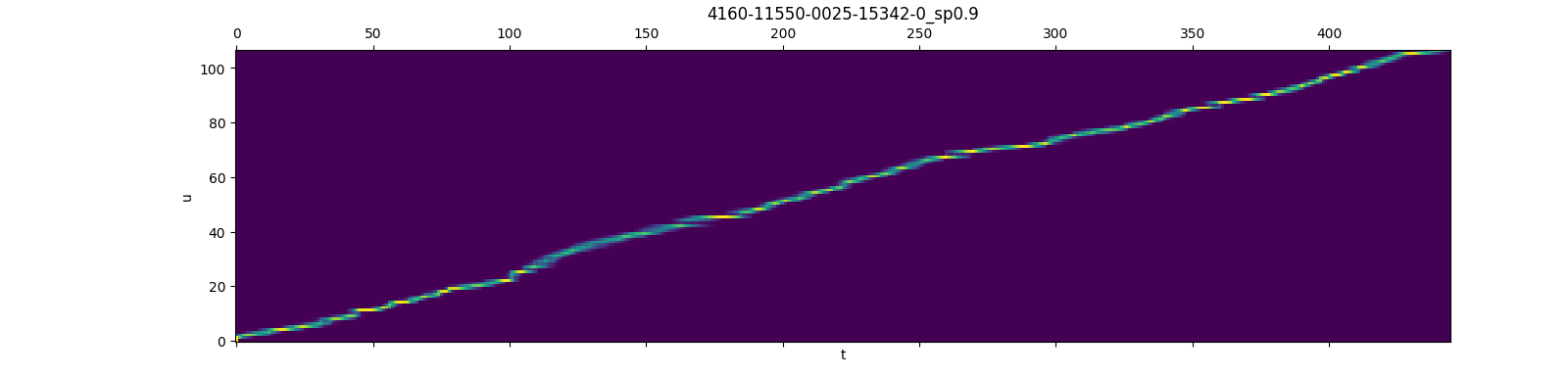
The following shows some plots for different utterances.

You can see that

• Most of the nodes have a very small gradient, i.e., most of the nodes have the background color.
• Positions of nodes with non-zero gradient change somewhat monotonically, from the lower left to the upper right
• At each time frame, only a small set of nodes have a non-zero gradient, which justifies the pruned RNN-T loss, i.e., putting a limit on the number of symbols per frame.

[csukuangfj]

This PR is not for merge. It is useful for visualizing the node gradient in the lattice during training.

[pkufool]

Are these pictures from the very first beginning steps or the stable training steps(i.e. middle steps at epoch 5 or other larger epochs).

[csukuangfj]

Note: The above plots are from the first batch at the very beginning of the training, i.e., the model weights are randomly initialized and no backward pass has been performed on it yet.

The following plots use the pre-trained model from https://github.com/k2-fsa/icefall/pull/248

[csukuangfj]

For better comparison, the plots between the model with randomly initialized weights and the pre-trained model are listed as follows:

Randomly initialized	Pre-trained

[desh2608]

@csukuangfj which quantity are you plotting here exactly? Is it simple_loss.grad?

[csukuangfj]

@csukuangfj which quantity are you plotting here exactly? Is it simple_loss.grad?

It is related to simple_loss, but it is not simple_loss.grad.

We are plotting the occupation probability of each node in the lattice. Please refer to the following code if you want to learn more.

• https://github.com/k2-fsa/icefall/blob/054e2399b9d21cbd1aac6186f80997f0eef2104f/egs/librispeech/ASR/pruned_transducer_stateless/model.py#L186
• https://github.com/k2-fsa/k2/blob/0d7ef1a7867f70354ab5c59f2feb98c45558dcc7/k2/python/k2/mutual_information.py#L395

    # this is a kind of "fake gradient" that we use, in effect to compute
    # occupation probabilities.  The backprop will work regardless of the
    # actual derivative w.r.t. the total probs.
    ans_grad = torch.ones(B, device=px_tot.device, dtype=px_tot.dtype)

    (px_grad,
     py_grad) = _k2.mutual_information_backward(px_tot, py_tot, boundary, p,
                                                ans_grad)

• https://github.com/k2-fsa/k2/blob/0d7ef1a7867f70354ab5c59f2feb98c45558dcc7/k2/python/csrc/torch/mutual_information_cpu.cu#L126

// backward of mutual_information.  Returns (px_grad, py_grad).
// p corresponds to what we computed in the forward pass.
std::vector<torch::Tensor> MutualInformationBackwardCpu(
    torch::Tensor px, torch::Tensor py,
    torch::optional<torch::Tensor> opt_boundary, torch::Tensor p,
    torch::Tensor ans_grad) {

I suggest that you derive the formula of the occupation probability of each node on your own. You can find the code at https://github.com/k2-fsa/k2/blob/0d7ef1a7867f70354ab5c59f2feb98c45558dcc7/k2/python/csrc/torch/mutual_information_cpu.cu#L189-L215

              // The s,t indexes correspond to
              // The statement we are backpropagating here is:
              // p_a[b][s][t] = LogAdd(
              //    p_a[b][s - 1][t + t_offset] + px_a[b][s - 1][t + t_offset],
              //    p_a[b][s][t - 1] + py_a[b][s][t - 1]);
              // .. which obtains p_a[b][s][t - 1] from a register.
              scalar_t term1 = p_a[b][s - 1][t + t_offset] +
                               px_a[b][s - 1][t + t_offset],
                       // term2 = p_a[b][s][t - 1] + py_a[b][s][t - 1], <-- not
                       // actually needed..
                  total = p_a[b][s][t];
              if (total - total != 0) total = 0;
              scalar_t term1_deriv = exp(term1 - total),
                       term2_deriv = 1.0 - term1_deriv,
                       grad = p_grad_a[b][s][t];
              scalar_t term1_grad, term2_grad;
              if (term1_deriv - term1_deriv == 0.0) {
                term1_grad = term1_deriv * grad;
                term2_grad = term2_deriv * grad;
              } else {
                // could happen if total == -inf
                term1_grad = term2_grad = 0.0;
              }
              px_grad_a[b][s - 1][t + t_offset] = term1_grad;
              p_grad_a[b][s - 1][t + t_offset] = term1_grad;
              py_grad_a[b][s][t - 1] = term2_grad;
              p_grad_a[b][s][t - 1] += term2_grad;

[desh2608]

Thanks for the detailed explanation!