scikit-learn
 scikit-learn copied to clipboard
FEA add Cholesky based Newton solver to GLMs
Reference Issues/PRs
Fixes #16634. #23619 should be merged first.
What does this implement/fix? Explain your changes.
This PR adds Newton solvers where the Newton step is obtained by a Cholesky decomposition. Another variant first uses a QR decomposition of X' which is beneficial for n_features >> n_samples.
This is basically the same as iterated reweighted least squares (IRLS) with inner Cholesky based solver on the normal equations.
Any other comments?
2 points:
- For now,
PoissonRegressor,GammaRegressorandTweedieRegressorhave the new solvers. It is very easy to extend it to binaryLogisticRegressionas well. - For now, there are 2 more solver options
"newton-cholesky"and"newton-qr-cholesky". These could finally be merged to a single one which automatically selects one based onn_samplesandn_features.
Based on our example from sklearn.linear_model import PoissonRegressor, see also #21787.
import numpy as np
from sklearn.compose import ColumnTransformer
from sklearn.datasets import fetch_openml
from sklearn.linear_model import PoissonRegressor
from sklearn.pipeline import make_pipeline
from sklearn.preprocessing import FunctionTransformer, OneHotEncoder
from sklearn.preprocessing import StandardScaler, KBinsDiscretizer


df = fetch_openml(data_id=41214, as_frame=True).frame
df["Frequency"] = df["ClaimNb"] / df["Exposure"]
log_scale_transformer = make_pipeline(
    FunctionTransformer(np.log, validate=False), StandardScaler()
)
linear_model_preprocessor = ColumnTransformer(
    [
        ("passthrough_numeric", "passthrough", ["BonusMalus"]),
        ("binned_numeric", KBinsDiscretizer(n_bins=10, subsample=None), ["VehAge", "DrivAge"]),
        ("log_scaled_numeric", log_scale_transformer, ["Density"]),
        (
            "onehot_categorical",
            OneHotEncoder(),
            ["VehBrand", "VehPower", "VehGas", "Region", "Area"],
        ),
    ],
    remainder="drop",
)
y = df["Frequency"]
w = df["Exposure"]
X = linear_model_preprocessor.fit_transform(df)
%time PoissonRegressor(solver="lbfgs", alpha=1e-4, tol=1e-4, max_iter=1000).fit(X, y); None
Wall time: 11.7 s
%time PoissonRegressor(solver="newton-cholesky", alpha=1e-4, tol=1e-4).fit(X, y); None
Wall time: 2.04 s
Note: On synthetic data (make_low_rank_matrix or make_regression), I often observe lbfgs to be faster, but on real data that is seldom the case in my experience.
Note to myself: For tiny alpha like 1e-12, it raises LinAlgWarning: Ill-conditioned matrix and the results disagree a little bit. lbfgs seems to find a solution with just a little smaller L2 norm than cholesky based.
Note to myself: For tiny alpha like 1e-12, it raises LinAlgWarning: Ill-conditioned matrix and the results disagree a little bit. lbfgs seems to find a solution with just a little smaller L2 norm than cholesky based.
Is there a thread-safe way to detect this situation and raise a higher level warnings that suggest to increase the regularization or use the "lbfgs" solver in this case?
Interesting benchmark results. I can reproduce locally. The "newton-cholesky" solver converged (with tol=1e-4) in 5 iterations while the "lbfgs" solver needs 506 iterations with the same tol value.
I am not sure the convergence criterion for both solver is the same though. I would be interesting to plot the final objective value on the training set vs n_iter_ or fit wall time for each solver for a logspaced grid of tol values in np.logspace(-8, -1, 8) and plot the results.
It seems that the LBFGS solver can get stuck and never converges exactly to the optimum (one order of magnitude above the solution found by the new solver) even for low tols.
Note to myself: For tiny alpha like 1e-12, it raises LinAlgWarning: Ill-conditioned matrix and the results disagree a little bit. lbfgs seems to find a solution with just a little smaller L2 norm than cholesky based.
Is there a thread-safe way to detect this situation and raise a higher level warnings that suggest to increase the regularization or use the "lbfgs" solver in this case?
PoissonRegressor(solver="newton-cholesky", alpha=1e-12, tol=1e-4).fit(X, y) raises—very thread safe—in every of its 5 iterations this LinAlgWarning, but it finally converges and has a slightly better loss function (by ~4.7e-6) than the lbfgs version.
callbacks would really be useful here.
You can set verbose to 1 or 2 and get very detailed information.
Concerning timing benchmarks: I have something in the pipe, where I first find tolerances that give comparable results. Unfortunately, syntactic data, even benchopt.datasets.make_correlated_data do not show the performance gap as seen in the french insurance claim dataset. On syntactic data, it's hard to beat lbfgs or I do something stupid.
Concerning timing benchmarks: I have something in the pipe, where I first find tolerances that give comparable results. Unfortunately, syntactic data, even benchopt.datasets.make_correlated_data do not show the performance gap as seen in the french insurance claim dataset. On syntactic data, it's hard to beat lbfgs or I do something stupid.
It would be interesting to understand what makes lbfgs comparatibely fail on this data. It's weird that it needs hundreds or even thousand of iterations to reach tol below 1e-7 on convex linear model fitting optimization problem. We could introspect the spectrum of the hessian at the optimum and maybe forge a synthetic quadratic optimization problem? Or maybe it's the evolution of the hessian on the optimization path that makes the problem hard for LBFGS to track?
Is this a result of the very noisy regression problem, possibly with significant heteroscedasticity?
Here are some notes from a first quick code review. As discussed with @GaelVaroquaux and @agramfort it would be interesting how this solver compares with an equivalent of the solver="newton-cg" implemented in LogisticRegression. The latter does not require materializing the hessian in memory.
Binary logistic regression on kick dataset
Things become really interesting for binary logistic regression. I chose the "kick" dataset, because it is comparable in size to the freMTPL2freq dataset. It has n_samples, n_features = 72983, 33.
Scripts
import numpy as np
import pandas as pd
from sklearn._loss import HalfBinomialLoss
from sklearn.compose import ColumnTransformer
from sklearn.datasets import fetch_openml
from sklearn.impute import SimpleImputer
from sklearn.linear_model._glm.glm import _GeneralizedLinearRegressor
from sklearn.linear_model._linear_loss import LinearModelLoss
from sklearn.linear_model import LogisticRegression
from sklearn.pipeline import make_pipeline
from sklearn.preprocessing import OneHotEncoder
from sklearn.preprocessing import StandardScaler


class BinomialRegressor(_GeneralizedLinearRegressor):
    def _get_loss(self):
        return HalfBinomialLoss()


df = fetch_openml(data_id=41162, as_frame=True).frame

linear_model_preprocessor = ColumnTransformer(
    [
        (
            "passthrough_numeric",
            make_pipeline(SimpleImputer(), StandardScaler()),
            [
                "MMRAcquisitionAuctionAveragePrice",
                "MMRAcquisitionAuctionCleanPrice",
                "MMRCurrentAuctionAveragePrice",
                "MMRCurrentAuctionCleanPrice",
                "MMRCurrentRetailAveragePrice",
                "MMRCurrentRetailCleanPrice",
                "MMRCurrentRetailAveragePrice",
                "MMRCurrentRetailCleanPrice",
                "VehBCost",
                "VehYear",
                "VehicleAge",
                "WarrantyCost",
            ],
        ),
        (
            "onehot_categorical",
            OneHotEncoder(min_frequency=10),
            [
                "Auction",
                "Color",
                "IsOnlineSale",
                "Make",
                "Model",
                "Nationality",
                "Size",
                "SubModel",
                "Transmission",
                "Trim",
                "WheelType",
            ],
        ),
    ],
    remainder="drop",
)
y = np.asarray(df["IsBadBuy"] == "1", dtype=float)
X = linear_model_preprocessor.fit_transform(df)
alpha = 1e-4
%time clf_lbfgs = LogisticRegression(solver="lbfgs", C=1 / alpha / X.shape[0], tol=1e-4, max_iter=1000).fit(X, y)
Wall time: 1.48 s
%time clf_newton_cg = LogisticRegression(solver="newton-cg", C=1 / alpha / X.shape[0], tol=1e-4, max_iter=1000).fit(X, y)
Wall time: 1.42 s
%time clf_lbfgs2 = BinomialRegressor(solver="lbfgs", alpha=alpha, tol=1e-4, max_iter=1000).fit(X, y)
Wall time: 478 ms
%time clf_newton_cholesky = BinomialRegressor(solver="newton-cholesky", alpha=alpha, tol=1e-4).fit(X, y)
Wall time: 781 ms
They achieve different losses
lml = LinearModelLoss(base_loss=HalfBinomialLoss(), fit_intercept=True)
sw = np.full_like(y, fill_value=1 / y.shape[0])
loss_lbfgs = lml.loss(coef=np.r_[clf_lbfgs.coef_[0], clf_lbfgs.intercept_], X=X, y=y, sample_weight=sw, l2_reg_strength=alpha)
loss_newton_cg = lml.loss(coef=np.r_[clf_newton_cg.coef_[0], clf_newton_cg.intercept_], X=X, y=y, sample_weight=sw, l2_reg_strength=alpha)
loss_lbfgs2 = lml.loss(coef=np.r_[clf_lbfgs2.coef_, clf_lbfgs2.intercept_], X=X, y=y, sample_weight=sw, l2_reg_strength=alpha)
loss_newton_cholesky = lml.loss(coef=np.r_[clf_newton_cholesky.coef_, clf_newton_cholesky.intercept_], X=X, y=y, sample_weight=sw, l2_reg_strength=alpha)
loss_newton_cg 0.3065839722555997 < loss_newton_cholesky 0.30658397857185354 < loss_lbfgs 0.306584001191482 < loss_lbfgs2 0.3066001389832086
Notes
- The LBFGS version of the BinomialRegressor uses
mean(loss)and"ftol": 64 * eps(this PR already set this much smaller) while the version ofLogisticRegressionusessum(loss)without the extraftoloption. This makes a difference! - Some solvers are quite allergic to omitting the
StandardScaler:"newton-cg"then needs 13s instead of 1.4s and raisesLineSearchWarning: The line search algorithm did not converge. But the final loss = 0.30698 is quite good.BinomialRegressor(solver="lbfgs") needs 5s, raisesConvergenceWarning: lbfgs failed to converge (status=1): STOP: TOTAL NO. of ITERATIONS REACHED LIMIT.Final loss = 0.31279 (not so good)LogisticRegression(solver="lbfgs")passes without warning in similar time as before. Final loss = 0.34987 is pretty bad.BinomialRegressor(solver="newton-cholesky")needs 1s (a little more than before) and raisesLinAlgWarning: Ill-conditioned matrix (rcond=2.35183e-17): result may not be accurate.Final loss = 0.30651 is clearly the best!
Things become really interesting for binary logistic regression.
Thanks! Those results are really interesting. One problem to interpret these is that it seems that the stopping criteria triggered in a different way.
With regards to Newton-cg vs Newton-cholesky: the difference should be marked in higher dimensions. It would be interesting to have a benchmark with p in the hundreds.
With regards to Newton-cg vs Newton-cholesky: the difference should be marked in higher dimensions. It would be interesting to have a benchmark with p in the hundreds.
X.shape = (72983, 1075)
X.shape = (72983, 1075)
OK, taking this back. Makes the benchmark very interesting.
Those experiments shed new lights on past discussions on LogisticRegression with lbfgs on ill-conditioned problems:
- #15583
There is also this attempt to use the related trust-ncg solver from scipy but:
- #22236
but it wasn't successful (at this point).
I ran some further benchmark on a imbalanced binarized variant of the original regression data to be able to compare with the binary classifiers of scikit-learn main.
I can reproduce the strong speed-up of the new "newton-cholesky" solver on this problem:
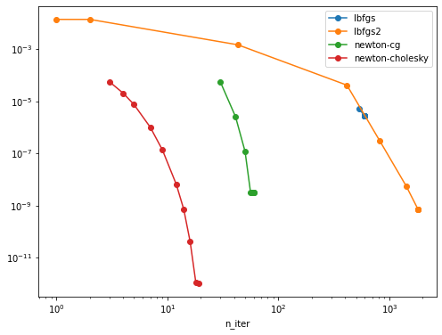
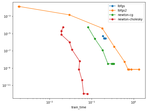
Here lbfgs2 stands for the LBFGS solver using the BinomialRegressor GLM.
To reproduce here are the scripts:
EDIT by @lorentzenchr: I corrected C = 2. / alpha / X.shape[0] to C = 1. / alpha / X.shape[0]. This does not change the plots (much).
import warnings
from pathlib import Path
import numpy as np
from sklearn.metrics import log_loss
from sklearn.compose import ColumnTransformer
from sklearn.datasets import fetch_openml
from sklearn.linear_model import LogisticRegression
from sklearn.pipeline import make_pipeline
from sklearn.preprocessing import FunctionTransformer, OneHotEncoder
from sklearn.preprocessing import StandardScaler, KBinsDiscretizer
from sklearn.exceptions import ConvergenceWarning
from sklearn.model_selection import train_test_split
from sklearn._loss import HalfBinomialLoss
from sklearn.linear_model._linear_loss import LinearModelLoss
from sklearn.linear_model._glm.glm import _GeneralizedLinearRegressor
from time import perf_counter
import pandas as pd
import joblib


class BinomialRegressor(_GeneralizedLinearRegressor):
    def _get_loss(self):
        return HalfBinomialLoss()


@joblib.Memory(location=".").cache
def prepare_data():
    df = fetch_openml(data_id=41214, as_frame=True).frame
    df["Frequency"] = df["ClaimNb"] / df["Exposure"]
    log_scale_transformer = make_pipeline(
        FunctionTransformer(np.log, validate=False), StandardScaler()
    )
    linear_model_preprocessor = ColumnTransformer(
        [
            ("passthrough_numeric", "passthrough", ["BonusMalus"]),
            (
                "binned_numeric",
                KBinsDiscretizer(n_bins=10, subsample=None),
                ["VehAge", "DrivAge"],
            ),
            ("log_scaled_numeric", log_scale_transformer, ["Density"]),
            (
                "onehot_categorical",
                OneHotEncoder(),
                ["VehBrand", "VehPower", "VehGas", "Region", "Area"],
            ),
        ],
        remainder="drop",
    )
    y = df["Frequency"]
    w = df["Exposure"]
    X = linear_model_preprocessor.fit_transform(df)
    return X, y, w


X, y, w = prepare_data()
y = y.values
y = (y > np.quantile(y, q=0.95)).astype(np.float64)
print(y.mean())


X_train, X_test, y_train, y_test, w_train, w_test = train_test_split(
    X, y, w, train_size=5_000, test_size=10_000, random_state=0
)
print(f"{X_train.shape = }")

results = []
loss_sw = np.full_like(y_train, fill_value=(1.0 / y_train.shape[0]))
# loss_sw = None
alpha = 1e-12
C = 1. / alpha / X.shape[0]
max_iter = 10_000
for tol in np.logspace(-1, -10, 10):
    for solver in ["lbfgs", "lbfgs2", "newton-cg", "newton-cholesky"]:
        tic = perf_counter()
        with warnings.catch_warnings():
            warnings.filterwarnings("ignore", category=ConvergenceWarning)
            if solver in ["lbfgs", "newton-cg"]:
                model = LogisticRegression(
                    C=C, solver=solver, tol=tol, max_iter=max_iter
                ).fit(X_train, y_train)
                toc = perf_counter()
            else:
                if solver == "lbfgs2":
                    binomial_solver = "lbfgs"
                else:
                    binomial_solver = solver
                model = BinomialRegressor(
                    solver=binomial_solver, alpha=alpha, tol=tol, max_iter=max_iter
                ).fit(X_train, y_train)
                toc = perf_counter()
        train_time = toc - tic

        lml = LinearModelLoss(base_loss=HalfBinomialLoss(), fit_intercept=True)
        train_loss = lml.loss(
            coef=np.r_[model.coef_.ravel(), model.intercept_.ravel()],
            X=X_train,
            y=y_train.astype(np.float64),
            sample_weight=loss_sw,
            l2_reg_strength=alpha,
        )
        result = {
            "solver": solver,
            "tol": tol,
            "train_time": train_time,
            "train_loss": train_loss,
            "n_iter": int(np.squeeze(model.n_iter_)),
            "converged": np.squeeze(model.n_iter_ < model.max_iter).all(),
            "coef_sq_norm": (model.coef_**2).sum(),
        }
        print(result)
        results.append(result)


results = pd.DataFrame.from_records(results)
results.to_csv(Path(__file__).parent / "bench_quantile_clf.csv")
and to plot the results (using the VS Code notebook-style cell separators):
# %%
import pandas as pd
from pathlib import Path

results = pd.read_csv(Path(__file__).parent / "bench_quantile_clf.csv")
results["suboptimality"] = results["train_loss"] - results["train_loss"].min() + 1e-12
results

# %%
import matplotlib.pyplot as plt

fig, ax = plt.subplots(figsize=(8, 6))
for label, group in results.groupby("solver"):
    group.sort_values("tol").plot(x="n_iter", y="suboptimality", loglog=True, marker="o", label=label, ax=ax)

# %%
import matplotlib.pyplot as plt

fig, ax = plt.subplots(figsize=(8, 6))
for label, group in results.groupby("solver"):
    group.sort_values("tol").plot(x="train_time", y="suboptimality", loglog=True, marker="o", label=label, ax=ax)
Here is the std output of the bench:
y.mean()=0.03441969401766633
X_train.shape = (5000, 75)
{'solver': 'lbfgs', 'tol': 0.1, 'train_time': 0.18598661499891023, 'train_loss': 0.1507104124597422, 'n_iter': 534, 'converged': True, 'coef_sq_norm': 148.5995818580439}
{'solver': 'lbfgs2', 'tol': 0.1, 'train_time': 0.0018889589991886169, 'train_loss': 0.16464095194724115, 'n_iter': 1, 'converged': True, 'coef_sq_norm': 8.189338530372188e-07}
{'solver': 'newton-cg', 'tol': 0.1, 'train_time': 0.08244384899990109, 'train_loss': 0.1507596083690232, 'n_iter': 30, 'converged': True, 'coef_sq_norm': 52.156190853890536}
{'solver': 'newton-cholesky', 'tol': 0.1, 'train_time': 0.021028338000178337, 'train_loss': 0.1507613498034356, 'n_iter': 3, 'converged': True, 'coef_sq_norm': 43.246954581859455}
{'solver': 'lbfgs', 'tol': 0.01, 'train_time': 0.20906995500081393, 'train_loss': 0.15070784765633458, 'n_iter': 597, 'converged': True, 'coef_sq_norm': 175.47327001538633}
{'solver': 'lbfgs2', 'tol': 0.01, 'train_time': 0.0018561130000307458, 'train_loss': 0.1646292901860732, 'n_iter': 2, 'converged': True, 'coef_sq_norm': 1.6951859649239628e-06}
{'solver': 'newton-cg', 'tol': 0.01, 'train_time': 0.11919979400045122, 'train_loss': 0.1507077390065617, 'n_iter': 41, 'converged': True, 'coef_sq_norm': 160.14747277515036}
{'solver': 'newton-cholesky', 'tol': 0.01, 'train_time': 0.019198382999093155, 'train_loss': 0.15072533002002153, 'n_iter': 4, 'converged': True, 'coef_sq_norm': 69.8043772595947}
{'solver': 'lbfgs', 'tol': 0.001, 'train_time': 0.1986105910000333, 'train_loss': 0.15070784765633458, 'n_iter': 597, 'converged': True, 'coef_sq_norm': 175.47327001538633}
{'solver': 'lbfgs2', 'tol': 0.001, 'train_time': 0.029593369999929564, 'train_loss': 0.1521817842828325, 'n_iter': 43, 'converged': True, 'coef_sq_norm': 7.5013732656079215}
{'solver': 'newton-cg', 'tol': 0.001, 'train_time': 0.18400128099892754, 'train_loss': 0.15070527795741132, 'n_iter': 50, 'converged': True, 'coef_sq_norm': 345.9929751427849}
{'solver': 'newton-cholesky', 'tol': 0.001, 'train_time': 0.01918990699959977, 'train_loss': 0.15071257151660727, 'n_iter': 5, 'converged': True, 'coef_sq_norm': 104.39093091285362}
{'solver': 'lbfgs', 'tol': 0.0001, 'train_time': 0.21090933900086384, 'train_loss': 0.15070784765633458, 'n_iter': 597, 'converged': True, 'coef_sq_norm': 175.47327001538633}
{'solver': 'lbfgs2', 'tol': 0.0001, 'train_time': 0.17953069299983326, 'train_loss': 0.1507467069057897, 'n_iter': 414, 'converged': True, 'coef_sq_norm': 60.06264818077148}
{'solver': 'newton-cg', 'tol': 0.0001, 'train_time': 0.24365168000076665, 'train_loss': 0.15070516219215194, 'n_iter': 56, 'converged': True, 'coef_sq_norm': 651.7428299174211}
{'solver': 'newton-cholesky', 'tol': 0.0001, 'train_time': 0.02997286200115923, 'train_loss': 0.15070616118837812, 'n_iter': 7, 'converged': True, 'coef_sq_norm': 197.91795799020952}
{'solver': 'lbfgs', 'tol': 1e-05, 'train_time': 0.20823906700024963, 'train_loss': 0.15070784765633458, 'n_iter': 597, 'converged': True, 'coef_sq_norm': 175.47327001538633}
{'solver': 'lbfgs2', 'tol': 1e-05, 'train_time': 0.344956529999763, 'train_loss': 0.1507054738069726, 'n_iter': 814, 'converged': True, 'coef_sq_norm': 341.3566737148675}
{'solver': 'newton-cg', 'tol': 1e-05, 'train_time': 0.3023405680014548, 'train_loss': 0.15070516205646955, 'n_iter': 58, 'converged': True, 'coef_sq_norm': 635.5151991524395}
{'solver': 'newton-cholesky', 'tol': 1e-05, 'train_time': 0.034281918000488076, 'train_loss': 0.15070529420603984, 'n_iter': 9, 'converged': True, 'coef_sq_norm': 323.958542199695}
{'solver': 'lbfgs', 'tol': 1e-06, 'train_time': 0.21524625399979413, 'train_loss': 0.15070784765633458, 'n_iter': 597, 'converged': True, 'coef_sq_norm': 175.47327001538633}
{'solver': 'lbfgs2', 'tol': 1e-06, 'train_time': 0.6079151290014124, 'train_loss': 0.15070516448290777, 'n_iter': 1417, 'converged': True, 'coef_sq_norm': 740.9214578134176}
{'solver': 'newton-cg', 'tol': 1e-06, 'train_time': 0.3186681099996349, 'train_loss': 0.15070516205646955, 'n_iter': 58, 'converged': True, 'coef_sq_norm': 635.5151991524395}
{'solver': 'newton-cholesky', 'tol': 1e-06, 'train_time': 0.05192724700100371, 'train_loss': 0.15070516539609255, 'n_iter': 12, 'converged': True, 'coef_sq_norm': 573.6390390498898}
{'solver': 'lbfgs', 'tol': 1e-07, 'train_time': 0.2077653360011027, 'train_loss': 0.15070784765633458, 'n_iter': 597, 'converged': True, 'coef_sq_norm': 175.47327001538633}
{'solver': 'lbfgs2', 'tol': 1e-07, 'train_time': 0.7390427080008521, 'train_loss': 0.15070515963328868, 'n_iter': 1816, 'converged': True, 'coef_sq_norm': 936.3705337077419}
{'solver': 'newton-cg', 'tol': 1e-07, 'train_time': 0.33580676699966716, 'train_loss': 0.1507051620561561, 'n_iter': 59, 'converged': True, 'coef_sq_norm': 635.5244500949951}
{'solver': 'newton-cholesky', 'tol': 1e-07, 'train_time': 0.05001377799999318, 'train_loss': 0.15070515966120773, 'n_iter': 14, 'converged': True, 'coef_sq_norm': 777.2120582392104}
{'solver': 'lbfgs', 'tol': 1e-08, 'train_time': 0.20477254599973094, 'train_loss': 0.15070784765633458, 'n_iter': 597, 'converged': True, 'coef_sq_norm': 175.47327001538633}
{'solver': 'lbfgs2', 'tol': 1e-08, 'train_time': 1.3517374439998093, 'train_loss': 0.15070515963328868, 'n_iter': 1816, 'converged': True, 'coef_sq_norm': 936.3705337077419}
{'solver': 'newton-cg', 'tol': 1e-08, 'train_time': 0.3325814299987542, 'train_loss': 0.1507051620561561, 'n_iter': 59, 'converged': True, 'coef_sq_norm': 635.5244500949951}
{'solver': 'newton-cholesky', 'tol': 1e-08, 'train_time': 0.05914708199998131, 'train_loss': 0.15070515898061512, 'n_iter': 16, 'converged': True, 'coef_sq_norm': 983.8925036892293}
{'solver': 'lbfgs', 'tol': 1e-09, 'train_time': 0.20599301099900913, 'train_loss': 0.15070784765633458, 'n_iter': 597, 'converged': True, 'coef_sq_norm': 175.47327001538633}
{'solver': 'lbfgs2', 'tol': 1e-09, 'train_time': 0.8797001679995446, 'train_loss': 0.15070515963328868, 'n_iter': 1816, 'converged': True, 'coef_sq_norm': 936.3705337077419}
/home/ogrisel/mambaforge/envs/dev/lib/python3.10/site-packages/scipy/optimize/_linesearch.py:415: LineSearchWarning: Rounding errors prevent the line search from converging
  warn(msg, LineSearchWarning)
/home/ogrisel/mambaforge/envs/dev/lib/python3.10/site-packages/scipy/optimize/_linesearch.py:305: LineSearchWarning: The line search algorithm did not converge
  warn('The line search algorithm did not converge', LineSearchWarning)
/home/ogrisel/code/scikit-learn/sklearn/utils/optimize.py:203: UserWarning: Line Search failed
  warnings.warn("Line Search failed")
{'solver': 'newton-cg', 'tol': 1e-09, 'train_time': 0.32125941199956287, 'train_loss': 0.1507051620561561, 'n_iter': 60, 'converged': True, 'coef_sq_norm': 635.5244500939592}
{'solver': 'newton-cholesky', 'tol': 1e-09, 'train_time': 0.06471875900024315, 'train_loss': 0.15070515894092798, 'n_iter': 18, 'converged': True, 'coef_sq_norm': 1089.436704012065}
{'solver': 'lbfgs', 'tol': 1e-10, 'train_time': 0.2037754640005005, 'train_loss': 0.15070784765633458, 'n_iter': 597, 'converged': True, 'coef_sq_norm': 175.47327001538633}
{'solver': 'lbfgs2', 'tol': 1e-10, 'train_time': 0.7767825829996582, 'train_loss': 0.15070515963328868, 'n_iter': 1816, 'converged': True, 'coef_sq_norm': 936.3705337077419}
/home/ogrisel/mambaforge/envs/dev/lib/python3.10/site-packages/scipy/optimize/_linesearch.py:415: LineSearchWarning: Rounding errors prevent the line search from converging
  warn(msg, LineSearchWarning)
/home/ogrisel/mambaforge/envs/dev/lib/python3.10/site-packages/scipy/optimize/_linesearch.py:305: LineSearchWarning: The line search algorithm did not converge
  warn('The line search algorithm did not converge', LineSearchWarning)
/home/ogrisel/code/scikit-learn/sklearn/utils/optimize.py:203: UserWarning: Line Search failed
  warnings.warn("Line Search failed")
{'solver': 'newton-cg', 'tol': 1e-10, 'train_time': 0.31698038700051256, 'train_loss': 0.1507051620561561, 'n_iter': 60, 'converged': True, 'coef_sq_norm': 635.5244500939592}
{'solver': 'newton-cholesky', 'tol': 1e-10, 'train_time': 0.07936050799980876, 'train_loss': 0.15070515894082342, 'n_iter': 19, 'converged': True, 'coef_sq_norm': 1094.996868879865}
Observations and comments
- both newton solvers fair better than both LBFGS solvers on this problem but the cholesky variant is still much better than the CG variant that does not explicitly materialize the Hessian matrix both from a wall-time point of view and from an
n_iterpoint of view: accurate Hessian estimation seems to be important for this problem - the difference is already significant for relatively small values of
n_samples(5000) butn_featuresis even smaller. - I have observed that for low tol values on more regularized problems the
newton-cgneed more than the budge of 10_000 iteration to converge: I suspect sensitivity to rounding errors that prevent it to converge for any value of max_iter. - the newton cholesky solver is more more stable comparatively.
- the lbfgs2 solver tend to warn with low tol values:
home/ogrisel/mambaforge/envs/dev/lib/python3.10/site-packages/scipy/optimize/_linesearch.py:415: LineSearchWarning: Rounding errors prevent the line search from converging
  warn(msg, LineSearchWarning)
/home/ogrisel/mambaforge/envs/dev/lib/python3.10/site-packages/scipy/optimize/_linesearch.py:305: LineSearchWarning: The line search algorithm did not converge
  warn('The line search algorithm did not converge', LineSearchWarning)
- the regular lbfgs solver in
LogisticRegressiondoes not seem to have this problem but the tol parametrization does not seem to be consistent and it never reaches low objective function values, even for the smallest tols - the two lbfgs solvers have different stopping criterions but their loss vs n_iter curve overlap
- I had to use a very low alpha value. For higher alpha values the curves do not really make sense, I am not sure the C vs alpha regularization parametrization is consistent for both kinds of models
I am further investigating issues related to the singular Hessian case in https://github.com/lorentzenchr/scikit-learn/pull/6.
With https://github.com/scikit-learn/scikit-learn/pull/23314/commits/e6684c6bd1c42074216fe6d8fe51f60caff05c2e, I completed the tests for unpenalized GLMs. Same as in #22910. Based on those, we can better investigate how to handle singular X with these Newton solvers.
The last commits contain substantial updates:
- https://github.com/scikit-learn/scikit-learn/pull/23314/commits/3fb36954b75492ee94f249ce0a6638cf48d2ed64 fixed the test around
glm_dataset. The GLM tests now take between 1-2 minutes (on my laptop). - I tried an SVD based fallback solver for singular hessians in https://github.com/scikit-learn/scikit-learn/pull/23314/commits/2b6485e001c7fbe7e3b0546af4ebd0f1c08c41d5. This did not work well and I reverted it.
- Finally, https://github.com/scikit-learn/scikit-learn/pull/23314/commits/d463817e97bc0d1a820c83c6fbec179c6d2b7fe0 uses simple gradient steps (using the diagonal elements of the hessian) for singular hessian and fixes the rest of the tests.
The new tests are very hard. I had to switch of TweedieRegressor(power=3.0) and TweedieRegressor(power=0, link="log"). Furthermore, https://github.com/scikit-learn/scikit-learn/pull/23314/commits/c9b120063574bdd9d408805ce96c34ebe7722f81 and https://github.com/scikit-learn/scikit-learn/pull/23314/commits/2f0ea15a2089861170b744e8a531708100c9ff88 introduce a fallback inner solver to 4 lbfgs iterations. This is handy for problems that have many negative pointwise hessian values. Alternatively, we could tell a solver to simply stop and raise a warning.
I did some experiments with synthetic Poisson data with independent yet all informative features on my side and found out that the difference between newton-cholesky and LBFGS is the biggest on datasets with a significant fraction (e.g. 1/3 but not all) of the features that are binary but with very rare 1. values (e.g. fewer than 0.1% on 100_000 or more samples).
I also noticed that the LBFGS solver is much slower (in terms of wall clock time) when X is a dense array instead of a CSR matrix compared to the other solvers where the physical representation does not impact the performance much on such data with only 1/3 of the features that are very sparse and the other that are 0 valued 50% of the time on average.
Those are interesting findings. The real datasets used above all have several categorical values which produce diagonal sub-blocks of the hessian. It seems lbfgs is just slower on those and newton-cholesky is just about the same as on other data (bottleneck is the matrix-matrix multiplication for the hessian, not the inner solver for the Newton step). I have no idea as to what causes the slow down of lbfgs.
I put the tests in a separate PR, #23619, to make this PR smaller once that is merged.
bottleneck is the matrix-matrix multiplication for the hessian, not the inner solver for the Newton step
Yes I did some profiling of the "newton-cholesky" solver and I arrived to the same conclusion. I was surprised that the line-search is very fast comparatively (and typically only require a single iteration).
I also profiled the "newton-lsmr" solver and the time is spent in the inner_solver step but this is expected because it implicitly forms the hessian during that step on the fly via the LinearOperator. The line search is also negligible.
I haven't yet found the time to investigate the surprisingly large performance impact of sparse vs dense for LBFGS (on data that is not that sparse).
This PR needs to be updated now that the GLM tests have been improved in main.
Furthermore, I suggested an alternative fallback mechanism for ill-conditioned problems in https://github.com/lorentzenchr/scikit-learn/pull/8.
I pushed a merged. I am not 100% sure of the rtol settings. I am running a local run with all random seeds.
I got some rtol related errors locally when running with the full random seeds. I will need to do another pass of tweaking but I don't have time to do it now.
@ogrisel I had a little time. Test tolerances are fixed in https://github.com/scikit-learn/scikit-learn/pull/23314/commits/5e6aa9974a862db813e1300d5cf0b47a6aed23a5. The fallback to lbfgs is done in ~~https://github.com/scikit-learn/scikit-learn/pull/23314/commits/5e6aa9974a862db813e1300d5cf0b47a6aed23a5~~ https://github.com/scikit-learn/scikit-learn/pull/23314/commits/d4206d68247ca1b439657be31ce9d86250a53d8a.
The fallback to lbfgs is done in https://github.com/scikit-learn/scikit-learn/commit/5e6aa9974a862db813e1300d5cf0b47a6aed23a5.
I guess you meant d4206d6. This is great, let me update my test PR accordingly.