xMIP

xMIP copied to clipboard

@raphaeldussin suggested some methods to fill/extrapolate coordinate values over at (https://github.com/xgcm/xgcm/issues/292#issuecomment-754751213) that might be better than the current logic used here.

This might help with #66 too.

I have experimented a bit with gridfill and HCtFlood but I am not sure that the results convince me.

I loaded the data that caused problems in #66:

# Load a cmip6 dataset with missing values in lon/lat
import xarray as xr
import intake
import matplotlib.pyplot as plt
import numpy as np

from cmip6_preprocessing.preprocessing import combined_preprocessing
url = "https://cmip6.storage.googleapis.com/pangeo-cmip6.json"

col = intake.open_esm_datastore(url)
model = 'CESM2-FV2'
query = dict(experiment_id=['historical'], table_id='Omon', 
             variable_id='tos', grid_label=['gn'], source_id=model)
cat = col.search(**query)
print(cat.df['source_id'].unique())
z_kwargs = {'consolidated': True, 'decode_times':False}
tos_dict = cat.to_dataset_dict(
    zarr_kwargs=z_kwargs,
    preprocess=None,
    aggregate=False
)
ds = tos_dict['CMIP.NCAR.CESM2-FV2.historical.r1i1p1f1.Omon.tos.gn.gs://cmip6/CMIP/NCAR/CESM2-FV2/historical/r1i1p1f1/Omon/tos/gn/.nan.20191120']

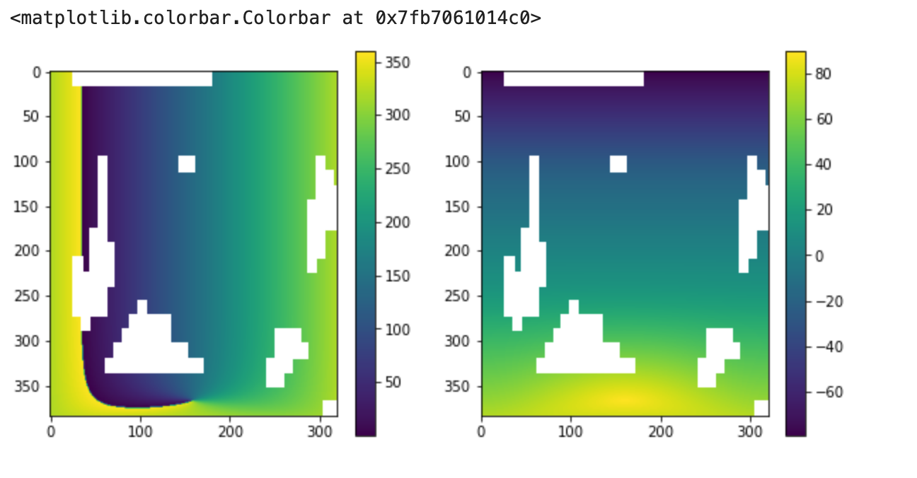
the lon and lat fields have missing values, which I mask out as nans

lon = ds.lon
lat = ds.lat
masked_lon = lon.where(lon<1000)
masked_lat = lat.where(lat<1000)

lon_data = masked_lon.load().data
lon_data_masked = np.ma.masked_array(data=lon_data, mask=np.isnan(lon_data))
lat_data = masked_lat.load().data
lat_data_masked = np.ma.masked_array(data=lat_data, mask=np.isnan(lat_data))

plt.figure(figsize=[10,5])
plt.subplot(1,2,1)
plt.imshow(lon_data_masked)
plt.colorbar()

plt.subplot(1,2,2)
plt.imshow(lat_data_masked)
plt.colorbar()

HCtFlood

import HCtFlood.kara as kara
lon_kara = ds.lon
lon_kara_filled = kara.flood_kara_ma(lon_data_masked, spval=1e35)
lat_kara = ds.lat
lat_kara_filled = kara.flood_kara_ma(lat_data_masked, spval=1e35)

plt.figure(figsize=[10,5])
plt.subplot(1,2,1)
plt.imshow(lon_kara_filled)
plt.colorbar()

plt.subplot(1,2,2)
plt.imshow(np.diff(lon_kara_filled, axis=1),vmin=0,vmax=2)
plt.colorbar()

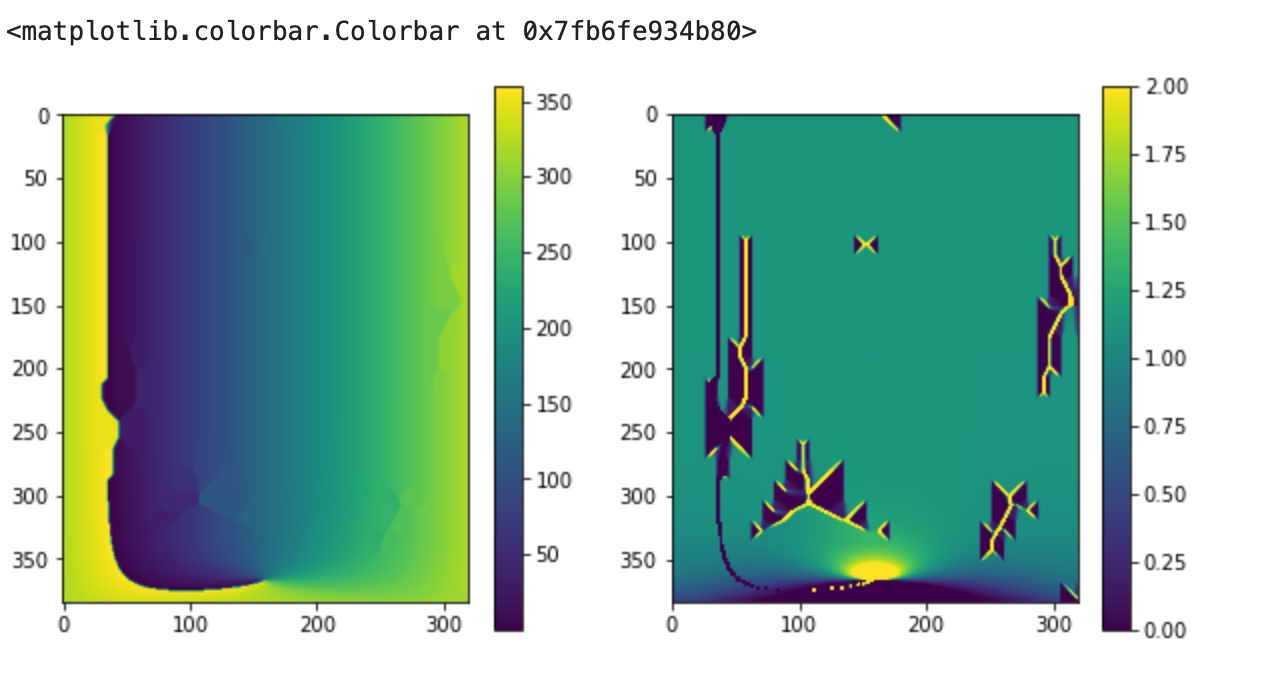
This doesnt look to bad visually, but you can see on the right that the longitude values are not monotonic, which causes all kind of issues with cartopy plotting

gridfill

import gridfill
filled_lon, converged_lon = gridfill.fill(lon_data_masked, 1, 0, 0.01, itermax=1e4, cyclic=True)
filled_lat, converged_lat = gridfill.fill(lat_data_masked, 1, 0, 0.01, itermax=1e4, cyclic=True)
print(converged_lon, converged_lat)

plt.figure(figsize=[10,5])
plt.subplot(1,2,1)
plt.imshow(filled_lon)
plt.colorbar()

plt.subplot(1,2,2)
plt.imshow(np.diff(filled_lon, axis=1),vmin=0,vmax=2)
plt.colorbar()

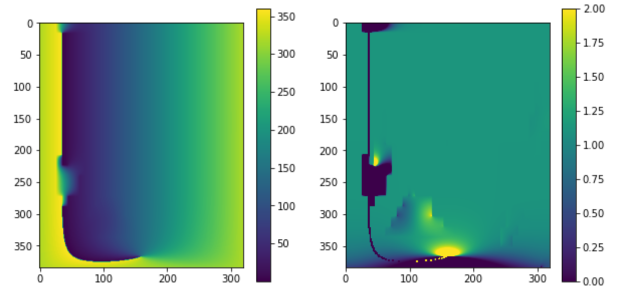
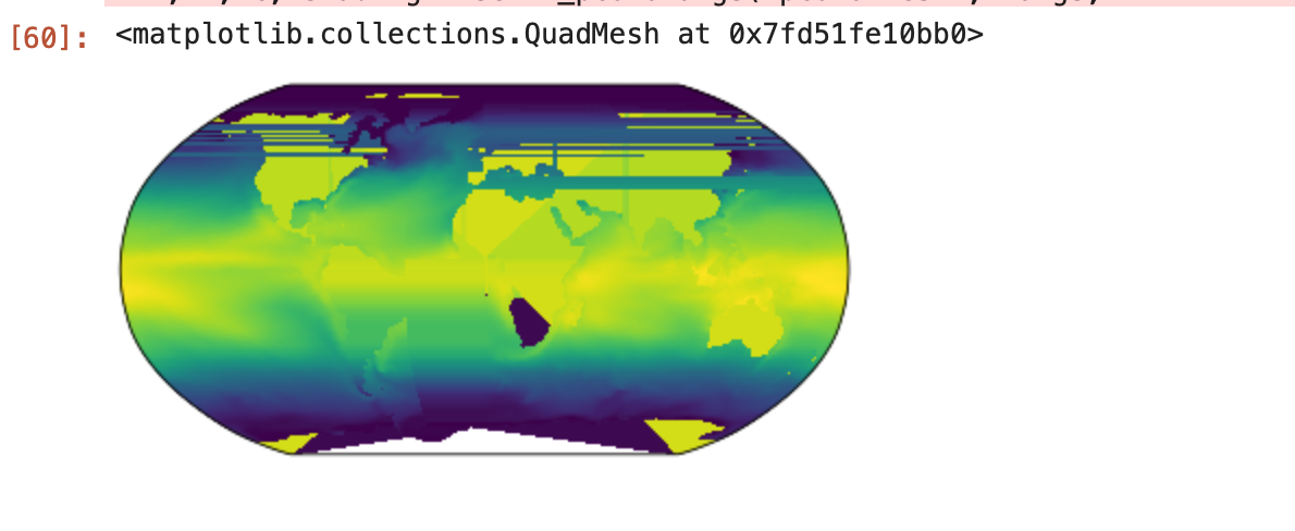
This looks great in all the areas that are not near the longitude discontinuity, but those non monotonic regions also seem to upset cartopy in a major fashion...

For now I am pretty sure that I do not want to make this step part of cmip6_preprocessing unless we can get this to work seemlessly with standard plotting methods.

I also have to admit I blindly used these methods without knowing much about them. If there are ways to tune the output, I would be very interested.

cc @raphaeldussin

yeah that does not work great, I wonder if it would be better with a combination of xarray.bfill and xarray.ffill along the axis perpendicular to the axis that varies most (i.e. y axis for lon, x for lat)

pop_tools has a lateral_fill algorithm you could try.

cc @ALDepp

Thanks for the tips. I will definitely come back to this later!