rTensor
 rTensor copied to clipboard
Randomized Tensor Decompositions
 Randomized CP Decomposition
The CP decomposition is an equation-free, data-driven tensor decomposition that is capable of providing accurate reconstructions of multi-mode data arising in signal processing, computer vision, neuroscience and elsewhere.
The ctensor package includes the following tensor decomposition routines:
- CP using the alternating least squares method (ALS)
- CP using the block coordinate descent method (BCD)
- Both methods can be used either using a deterministic or a fast randomized algorithm.
- The package is build ontop of the scikit-tensor package
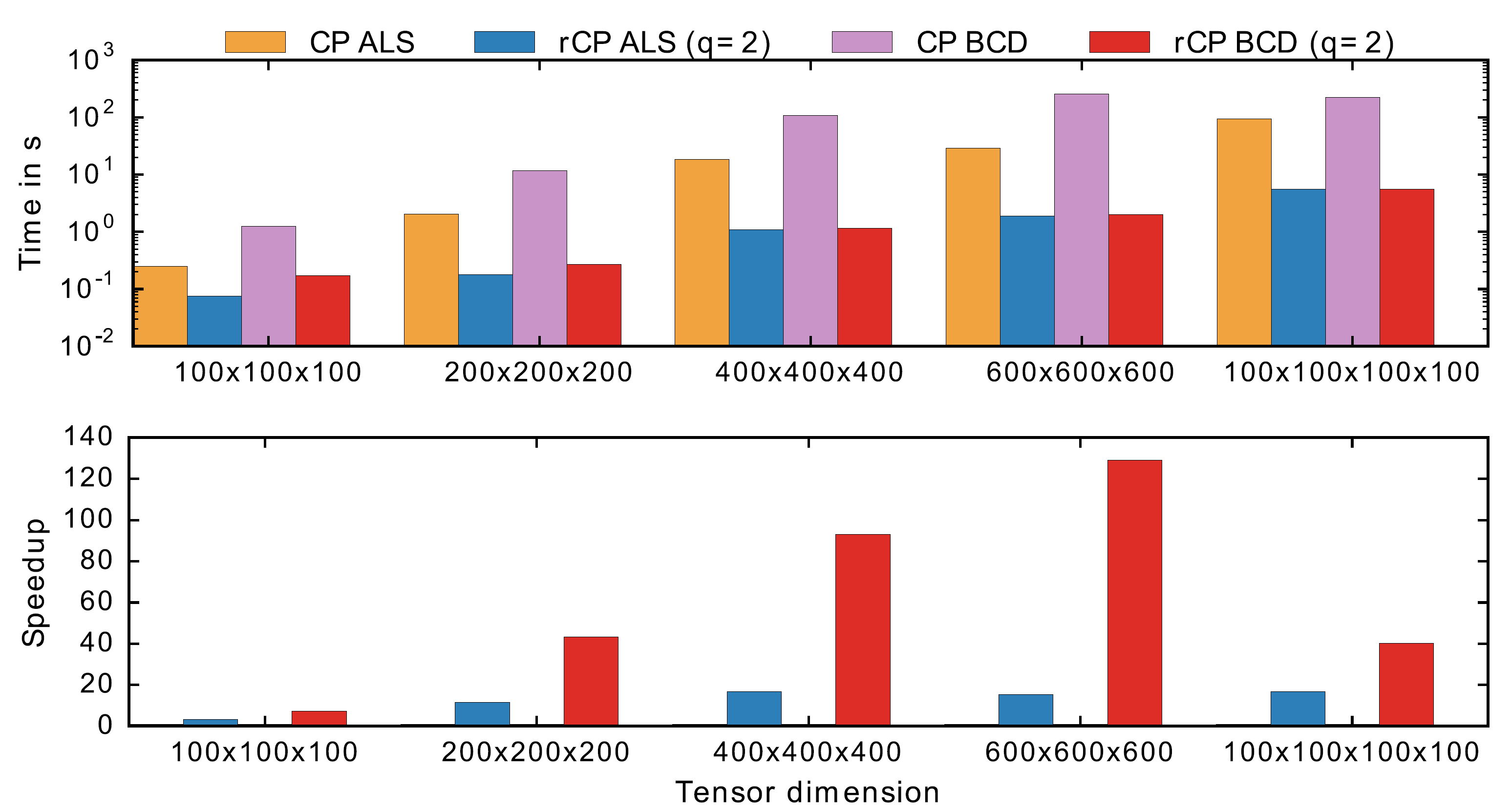
The following figure illustrates the performance of the randomized accelerated CP decomposition routines.
Installation
Get the latest version
git clone https://github.com/Benli11/ctensor
To build and install ctensor, run from within the main directory in the release:
python setup.py install
After successfully installing, the unit tests can be run by:
python setup.py test
See the documentation for more details (coming soon).
Example
Get started:
import numpy as np
from ctensor import ccp_als, ccp_bcd
from ctensor import dtensor, ktensor
First, lets create some toy data:
from ctensor import toydata
X = toydata(m=250, t=150, background=0, display=1)
This function returns a array of dimension 250x250x150, where the last index denotes time.
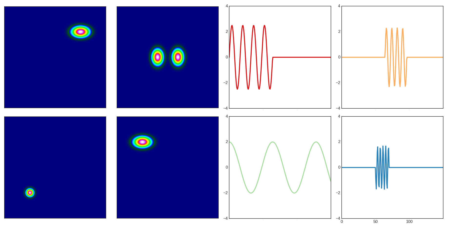
The underlying spatial modes and time dynamics of the data are shown in the following figure.
Then we define the array as a tensor as follows
T = dtensor(X)
The CP decomposition using the block coordine descent method (BCD) is obtained as
P = ccp_bcd(T , r=4, c=False, maxiter=500)
However, the deterministic algorihm is computational expensive in general. More efficently the randomized CP decompsition algorithm can be use to obtain a near-optimal approximation
P = ccp_bcd(T , r=4, c=True, p=10, q=2, maxiter=500)
where the parameter p denotes the amount of oversampling, and q denotes the number of additional power iterations. By, default we use p=10, and q=2 which are a good trade-off between computational speed and approximation quality. Once the CP decompostion is obtained, the lambda values and the factor matrices can be obtained as
print(P.lmbda)
A,B,C = P.U
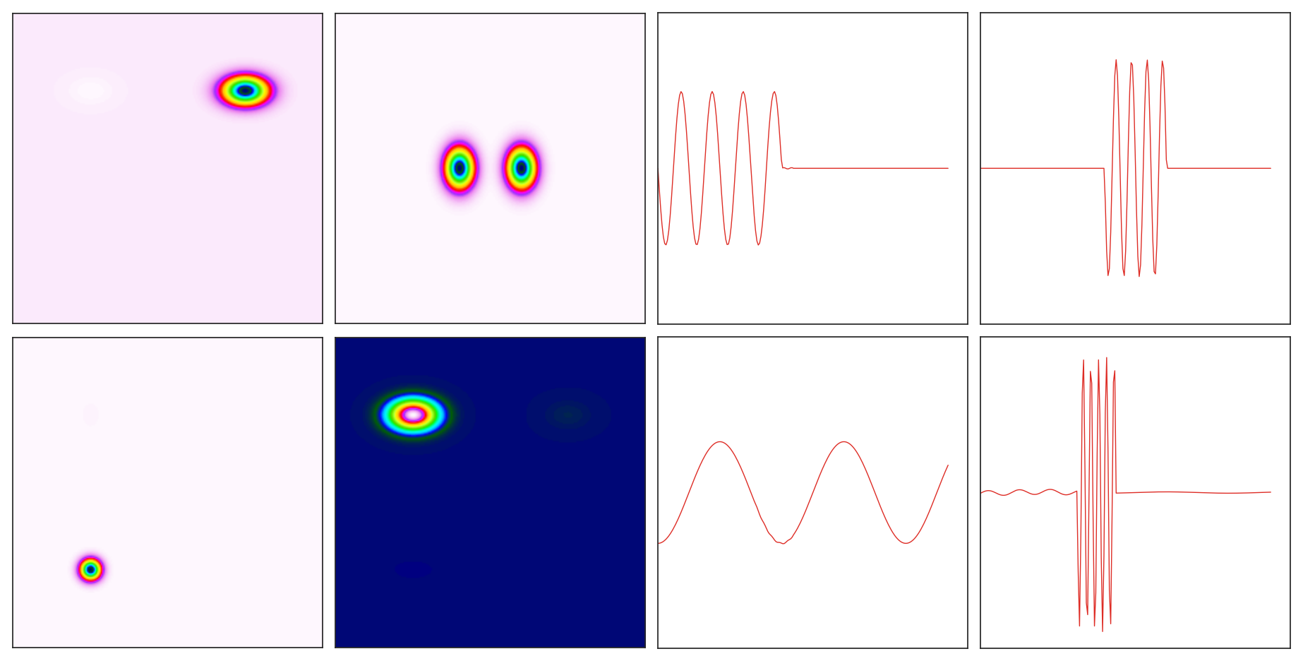
The next figure shows the reconstructed modes and time dynamics, which faithfully capture the underlying system.
References
- N. Benjamin Erichson, et al. “Randomized CP Tensor Decomposition.” (2016)
- Tamara G. Kolda and Brett W. Bader “Tensor Decompositions and Applications.” (2009)
- Nathan Halko, et al. “Finding structure with randomness: Probabilistic algorithms for constructing approximate matrix decompositions.” (2011)
- N. Benjamin Erichson, et al. “Randomized Matrix Decompositions using R.” (2016)