MetPy

MetPy copied to clipboard

Description Of Changes

Move toward using virtual temperature for the parcel profile instead of temperature

Closes #461

Checklist

• [ ] Closes #461
• [ ] Tests added
• [ ] Fully documented

While the tests are still failing (due to changing values) I would be interested to get feedback from @dopplershift / @jthielen on this approach... does this make sense? I tried to implement approaches discussed over in #461 ...

I would much rather get this fixed here instead of the downstream approach we have in ACT...

@mgrover1 I don't want to let this go too long without a response, but generally supportive of the approach. My first concern is making sure we get all the math right, which I haven't had a chance to sit down and make sure it all makes sense.

My other concern is making sure we can easily plumb this into all the places that need this knowledge for consistency.

@mgrover1 I don't want to let this go too long without a response, but generally supportive of the approach. My first concern is making sure we get all the math right, which I haven't had a chance to sit down and make sure it all makes sense.

My other concern is making sure we can easily plumb this into all the places that need this knowledge for consistency.

Thanks @dopplershift - I can put together some direct comparisons with the current method vs. the approach here, and look for a potential test case to make sure the math works out...

An Update

I put together a comparison of the implementation here compared to one currently in MetPy main

MetPy Main Branch

Surface-based CAPE: ~ 2329.4J/kg Surface-based CIN: ~ -92.32 J/kg

This PR (using virtual temperature)

Surface-based CAPE: ~ 2720.4J/kg Surface-based CIN: 0 J/kg

Is this right?

Graphically, this seems like the right approach, and takes into account the previous comments on this PR/related issues. What do people think? One thing to note here is that this will change the CAPE/CIN values in the testing suite, so we should either set the default value in the testing suite for whether to use the virtual temperature to be False, or the entire CAPE/CIN testing suite will need to be updated.

This still doesn't look correct. I'd have to take a look at the code, but from just looking at the plot above, the LCL should not be any different from the original uncorrected profile. It looks like you are using the virtual temperature at the surface in place of the regular temperature, and then lifting the parcel accordingly. This is leading to a higher LCL, and if so it's the wrong approach. (EDIT: yes, this appears to be what is happening - see my comments on the code below). Instead, the parcel should be lifted using the regular surface temperature as before, but then (and this is the crucial part), the resulting parcel temperature profile should be corrected using the virtual temperature. That is, compute the virtual temperature of the parcel given the parcel temp and dewpoint profile. then pass that profile into the CAPE calculation. Hopefully that makes sense.

Forgot the other part. When passing in the parcel virtual temp profile to the CAPE calculation, it should be compared against the environmental virtual temperature profile, not the environmental regular temperature profile. It looks like you are doing that though.

@mgrover1, I should be clear that I appreciate that you are taking the initiative here, and hope I'm not coming across as overly pedantic.

@Meteodan It's definitely appreciated to have the review of someone with intimate knowledge of what to expect.

@Meteodan agreed! Thank you for the helpful input here!!

@Meteodan I made those changes you suggested (I think) and this is the resultant SkewT diagram, highlighting the parcel profile and shaded CAPE... this doesn't look right either.

I think I am more confused than before...

and here is the code block changed

def _parcel_profile_helper(pressure, temperature, dewpoint,
                           assumptions=ParcelPathAssumptions()):
    """Help calculate parcel profiles.

    Returns the temperature and pressure, above, below, and including the LCL. The
    other calculation functions decide what to do with the pieces.

    """
    # Check that pressure does not increase.
    if not _check_pressure(pressure):
        msg = """
        Pressure increases between at least two points in your sounding.
        Using scipy.signal.medfilt may fix this."""
        raise InvalidSoundingError(msg)

    # Find the LCL
    press_lcl, temp_lcl = lcl(pressure[0], temperature, dewpoint)
    press_lcl = press_lcl.to(pressure.units)

    # Find the dry adiabatic profile, *including* the LCL. We need >= the LCL in case the
    # LCL is included in the levels. It's slightly redundant in that case, but simplifies
    # the logic for removing it later.
    press_lower = concatenate((pressure[pressure >= press_lcl], press_lcl))
    temp_lower = dry_lapse(press_lower, temperature)

    # Do the virtual temperature correction for the parcel below the LCL
    if assumptions.use_virtual_temperature:
        # Calculate the relative humidity, mixing ratio, and virtual temperature
        rh_lowest = relative_humidity_from_dewpoint(temperature, dewpoint)
        rv_lower = mixing_ratio_from_relative_humidity(press_lower[0], temperature, rh_lowest)
        temp_lower = virtual_temperature(temp_lower, rv_lower).to(temp_lower.units)
        temp_lcl = virtual_temperature(temp_lcl, rv_lower)

    # If the pressure profile doesn't make it to the lcl, we can stop here
    if _greater_or_close(np.nanmin(pressure), press_lcl):
        return (press_lower[:-1], press_lcl, units.Quantity(np.array([]), press_lower.units),
                temp_lower[:-1], temp_lcl, units.Quantity(np.array([]), temp_lower.units))

    # Establish profile above LCL
    press_upper = concatenate((press_lcl, pressure[pressure < press_lcl]))

    # Remove duplicate pressure values from remaining profile. Needed for solve_ivp in
    # moist_lapse. unique will return remaining values sorted ascending.
    unique, indices, counts = np.unique(press_upper.m, return_inverse=True, return_counts=True)
    unique = units.Quantity(unique, press_upper.units)
    if np.any(counts > 1):
        warnings.warn(f'Duplicate pressure(s) {unique[counts > 1]:~P} provided. '
                      'Output profile includes duplicate temperatures as a result.')

    # Find moist pseudo-adiabatic profile starting at the LCL, reversing above sorting
    temp_upper = moist_lapse(unique[::-1], temp_lower[-1]).to(temp_lower.units)
    temp_upper = temp_upper[::-1][indices]

    # Do the virtual temperature correction for the parcel above the LCL
    if assumptions.use_virtual_temperature:

        # Calculate the mixing ratio and virtual temperature
        rv_upper = mixing_ratio(saturation_vapor_pressure(temp_upper), press_upper)
        temp_upper = virtual_temperature(temp_upper, rv_upper).to(temp_lower.units)

    # Return profile pieces
    return (press_lower[:-1], press_lcl, press_upper[1:],
            temp_lower[:-1], temp_lcl, temp_upper[1:])

Don't correct the parcel profile until after the whole thing is computed. Here you are computing the lower part of the profile, then correcting it, then computing the upper part based on the corrected lower part, and then correcting the upper part. This is leading to the bizarre behavior near and above the LCL. Instead, compute both the lower and upper parts before the correction, and then apply the virtual temp correction to the whole thing.

Ahhh that makes more sense... I will give that a try! Sorry for the confusion here... thermo is slowly coming back :)

The classic paper on this subject contains a few soundings that could be used as additional test cases, assuming the Wyoming server has them.

The classic paper on this subject contains a few soundings that could be used as additional test cases, assuming the Wyoming server has them.

Thanks!! This is a great resource.

Think of it this way.... as far as the parcel is concerned, as it is lifted, its temperature will change based on the dry and moist adiabatic lapse rates. It's virtual temperature is just "along for the ride". The virtual temperature doesn't matter for the actual thermodynamics of the parcel behavior; it is only a diagnostic quantity that is a convenient way to incorporate the impact of water vapor on the density. The only time the virtual temperature matters here is when computing the CAPE because CAPE is the vertical integral of the buoyancy:

$B\approx -g\frac{\rho'}{\rho_{env}}\approx g\frac{T_v'}{T_{env}}=g\frac{T_{v,parcel}-T_{v,env}}{T_{v,env}}$

EDITED to correct formula for buoyancy (was in a hurry and forgot to multiply by g as well as the minus sign when using the density perturbation/environmental density)

This is why you should use the original parcel T and Td to compute its profile, including the dry adiabatic layer below the LCL, the LCL itself, and the moist adiabatic profile above. That's the true parcel temperature as it rises (assuming parcel theory is correct, of course). The virtual temperature of the parcel can then be computed at each level knowing the T and Td. It's this virtual temperature (ie. "corrected") profile that is passed (along with the environment's virtual temperature profile) to the CAPE routine to compute the CAPE with the "correction". FWIW, I don't like the word "correction" in this context. Really what we are doing is making a more accurate calculation of CAPE that includes the effect of water vapor on the density of the parcel and environment, and thus, the buoyancy.

The classic paper on this subject contains a few soundings that could be used as additional test cases, assuming the Wyoming server has them.

Yes, I was going to link to that. Thanks! Also, Chuck Doswell has a good write-up on these concepts here: http://www.flame.org/~cdoswell/virtual/virtual.html

In particular, section 4 is very relevant here.

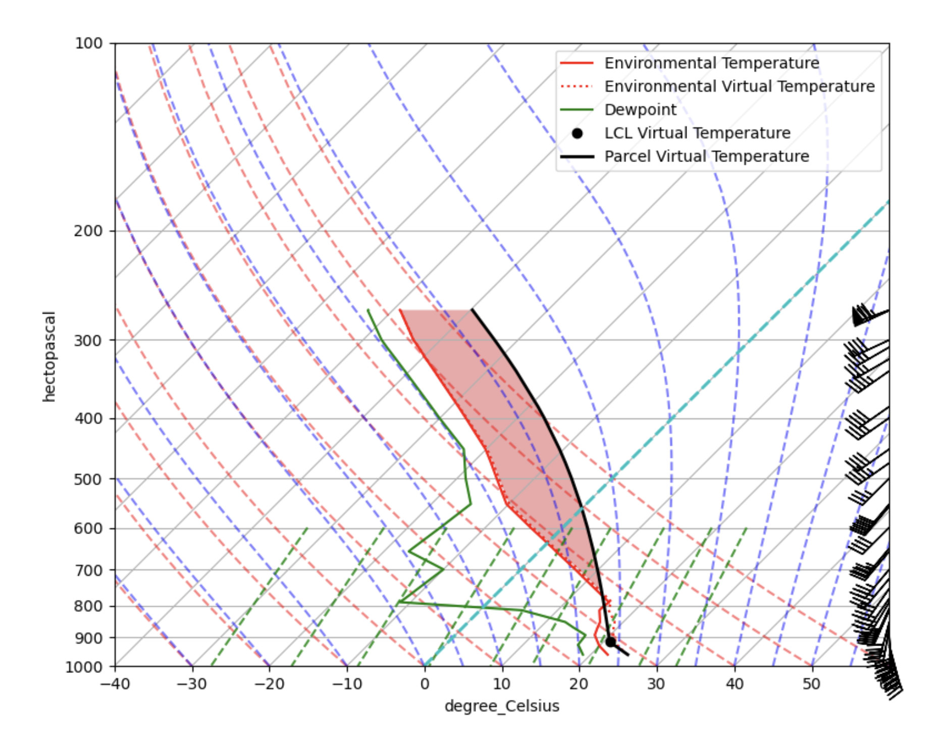
Following those suggestions of computing Tv after the fact, this is the result:

Looks good!

The classic paper on this subject contains a few soundings that could be used as additional test cases, assuming the Wyoming server has them.

I calculated the CAPE from these soundings, and the values are not nearly as high as the values described in the paper. I think they may have used additional sounding sites besides the NWS soundings, or additional QC/QA were added...

Here is a link to the Wallops sounding https://weather.uwyo.edu/cgi-bin/sounding?region=naconf&TYPE=TEXT%3ALIST&YEAR=1992&MONTH=08&FROM=1200&TO=1212&STNM=72402

From the sounding:

Station information and sounding indices Station identifier: WAL Station number: 72402 Observation time: 920812/0000 Station latitude: 37.93 Station longitude: -75.48 Station elevation: 12.0 Showalter index: 0.18 Lifted index: -8.64 LIFT computed using virtual temperature: -9.88 SWEAT index: 209.02 K index: 32.50 Cross totals index: 19.50 Vertical totals index: 27.50 Totals totals index: 47.00 Convective Available Potential Energy: 3632.90 CAPE using virtual temperature: 3940.76 Convective Inhibition: -10.98 CINS using virtual temperature: -10.52 Equilibrum Level: 151.12 Equilibrum Level using virtual temperature: 151.10 Level of Free Convection: 904.45 LFCT using virtual temperature: 908.06 Bulk Richardson Number: 207.03 Bulk Richardson Number using CAPV: 224.57 Temp [K] of the Lifted Condensation Level: 296.24 Pres [hPa] of the Lifted Condensation Level: 935.50 Equivalent potential temp [K] of the LCL: 359.59 Mean mixed layer potential temperature: 301.95 Mean mixed layer mixing ratio: 19.46 1000 hPa to 500 hPa thickness: 5754.00 Precipitable water [mm] for entire sounding: 49.51

where the CAPE values are estimated to be around ~3800 J/kg, but the paper states the values should be in excess of 4300 J/kg.

I wouldn't expect exact agreement in the numerical value of the CAPE, as it depends on other details of the calculation in addition to whether or not virtual temperature is used. For instance, is the latent heat of vaporization a constant, or is it allowed to vary with temperature? If it's a constant, what value of the constant is used? That affects the moist adiabatic lapse rate and thus the temperature profile of the parcel. There is also the choice of using the moist adiabatic lapse rate to compute the trajectory (essentially integrating the lapse rate with height), or computing theta-e at the LCL, and using that constant to define the trajectory above the LCL. That method in turn depends on which method you use to compute theta-e. So I'm guessing the Wyoming software is doing it one way, the software used in the article does it some other way, and perhaps MetPy yet a third way, and each way is going to give somewhat different results.

I wouldn't expect exact agreement in the numerical value of the CAPE, as it depends on other details of the calculation in addition to whether or not virtual temperature is used. For instance, is the latent heat of vaporization a constant, or is it allowed to vary with temperature? If it's a constant, what value of the constant is used? That affects the moist adiabatic lapse rate and thus the temperature profile of the parcel. There is also the choice of using the moist adiabatic lapse rate to compute the trajectory (essentially integrating the lapse rate with height), or computing theta-e at the LCL, and using that constant to define the trajectory above the LCL. That method in turn depends on which method you use to compute theta-e. So I'm guessing the Wyoming software is doing it one way, the software used in the article does it some other way, and perhaps MetPy yet a third way, and each way is going to give somewhat different results.

Yeah... that is a good point! I was hoping we could have a solid benchmark, a "truth" value :)

Alrighty - @dopplershift I went through and applied the suggestions discussed Friday, and updated the test suite... values for CAPE/such did not change by a huge amount but there were noticeable differences.

Where should we update the docs to reflect these changes? Some "as of 1.x.x version, virtual temperature is used"... do we need a more thorough explanation of why?

@Meteodan and I were chatting about it a few days ago. I just wanted to make sure that this was implemented such that it can be used for CAPE calculations as well as plotting capabilities. For instance, using the cape calculation is obviously important numerically, but plotting the virtually corrected profile is also important to understand the the distribution of CAPE as well. Just making sure this implementation will work for both.

@Meteodan and I were chatting about it a few days ago. I just wanted to make sure that this was implemented such that it can be used for CAPE calculations as well as plotting capabilities. For instance, using the cape calculation is obviously important numerically, but plotting the virtually corrected profile is also important to understand the the distribution of CAPE as well. Just making sure this implementation will work for both.

We can definitely add an example using the virtual temperature, instead of air temperature. I am not sure we want to re-implement logic in the profile calculation itself, but rather be explicit that we are converting to virtual temperature and plotting that. Would that make sense?

If I'm reading the test cases properly, for instance

-    (<Quantity(4578.94162, 'joule / kilogram')>, <Quantity(0, 'joule / kilogram')>)
+    (<Quantity(4550.1526, 'joule / kilogram')>, <Quantity(0, 'joule / kilogram')>)

using virtual temperature is decreasing the CAPE? I would expect almost always there would be an increase, since in the positive area, the parcel is saturated, but the environment in general is not, so Tv-T for the parcel should be larger than Tv-T for the environment, and therefore Tv(parcel) - Tv(environment) should be larger in the integrand for CAPE than T(parcel)-T(environment) is.

using virtual temperature is decreasing the CAPE? I would expect almost always there would be an increase, since in the positive area, the parcel is saturated, but the environment in general is not, so Tv-T for the parcel should be larger than Tv-T for the environment, and therefore Tv(parcel) - Tv(environment) should be larger in the integrand for CAPE than T(parcel)-T(environment) is.

@sgdecker This is the parcel being used here

Graphically, it appears that CAPE would be slightly less... I think if we had the full profile (all the way to the EL), CAPE would be greater, but since we are using part of the full profile, it might be less... do you have a suggestion on where the code is incorrect? It could just be a weird edge case.

Can you add the parcel temperature to that plot? This actually looks fairly similar to Fig. 2.9 in the Markowski textbook, where CAPE increases from 2872 J/kg to 3108 J/kg, and CIN decreases from 35 J/kg to 1 J/kg, when the virtual temperature is used. On p. 33, the text notes "In typical daytime temperature and moisture profiles, CAPE (CIN) values are increased (decreased) when the effects of moisture [i.e., virtual temperature] are included." which is in line with my expectations.

I'm not sure when/if I'll have a chance to look through this code to see if I notice anything there. Hopefully by the end of this week, but I can't make any promises.

I wonder if the issues is this line, where the dewpoint is the dewpoint of the environment and not the dewpoint of the parcel... would we need to calculate the parcel dewpoint separately?

parcel_profile = virtual_temperature_from_dewpoint(pressure, parcel_profile, dewpoint)

Would the dewpoint = temperature above the LCL? (sorry if that is a silly question) @sgdecker @Meteodan

@sgdecker

using virtual temperature is decreasing the CAPE? I would expect almost always there would be an increase

That was my intuition too, but I (incorrectly) managed to convince myself that it was ok. Your reasoning there makes much more sense, though.

@mgrover1

Would the dewpoint = temperature above the LCL? (sorry if that is a silly question) @sgdecker @Meteodan

That should be right since you get the LCL by having that state and it persists as the parcel rises. At any rate, suggest implementing that change and verifying that it largely just increases our CAPE values.