Hyperparameters-Optimization
 Hyperparameters-Optimization copied to clipboard
Hyperparameters-Optimization

- 하이퍼 파라미터 조정은 모든 기계 학습 프로젝트의 필수 부분이며 가장 시간이 많이 걸리는 작업 중 하나입니다.
- 가장 단순한 모델의 경우에도 하루, 몇 주 또는 그 이상 최적화 할 수있는 신경망을 언급하지 않고 최적의 매개 변수를 찾는 데 몇 시간이 걸릴 수 있습니다.
- 이 튜토리얼에서는 Grid Search , Random Search, HyperBand, Bayesian optimization, Tree-structured Parzen Estimator(TPE)에 대해 소개합니다.
- 하이퍼 파라미터 조정은 함수 최적화 작업에 지나지 않습니다. 그리고 분명히 Grid 또는 Random Search가 유일하고 최상의 알고리즘은 아니지만 효율적인 속도와 결과 측면에서 꾸준히 사용됩니다.
- 이론적 관점에서 어떻게 작동하는지 설명하고 Hyperopt 라이브러리를 사용하여 실제로 사용하는 방법을 보여줄 것입니다.
- 이 튜토리얼을 마치면 모델링 프로세스의 속도를 쉽게 높이는 방법을 알게됩니다.
- 튜토리얼의 유일한 목표는 매우 단순화 된 예제에서 Hyperparameter optimization을 사용하는 방법을 시연하고 설명하는 것입니다.
국내관련발표기고
- http://www.itdaily.kr/news/articleView.html?idxno=210339
- https://www.comworld.co.kr/news/articleView.html?idxno=50677
#!pip install pip install git+https://github.com/darenr/scikit-optimize
Preparation step
- 표준 라이브러리를 가져 옵니다
#!pip install lightgbm
import numpy as np
import pandas as pd

from lightgbm.sklearn import LGBMRegressor
from sklearn.metrics import mean_squared_error

%matplotlib inline

import warnings                                  # `do not disturbe` mode
warnings.filterwarnings('ignore')
sklearn.datasets의 당뇨병 데이터 세트에 대한 다양한 알고리즘을 시연하고 비교합니다. 로드합시다.
여기에서 데이터 세트에 대한 설명을 찾을 수 있습니다. [https://www4.stat.ncsu.edu/~boos/var.select/diabetes.html] add: 일부 환자 및 대상 측정 항목에 대한 정보가 포함 된 데이터 세트입니다. "기준선 1 년 후 질병 진행의 정량적 측정". 이 예제의 목적을 위해 데이터를 이해할 필요도 없습니다. 회귀 문제를 해결하고 있으며 하이퍼 파라미터를 조정하려고한다는 점을 명심하십시오.
from sklearn.datasets import load_diabetes

diabetes = load_diabetes()
n = diabetes.data.shape[0]

data = diabetes.data
targets = diabetes.target
- 데이터 세트는 매우 작습니다.
- 이를 사용하여 기본 개념을 쉽게 보여줄 수 있기 때문에 선택했습니다.( 모든 것이 계산 될 때 몇 시간을 기다릴 필요가 없습니다.)
- 데이터 세트를 학습 및 테스트 부분으로 나눌 것입니다. train 부분은 2 개로 분할되며, 매개 변수를 최적화하는 데 따라 교차 검증 MSE를 최종 측정 항목으로 사용할 것입니다.
add :이 간단한 예제는 실제 모델링을 위한 방법이 아닙니다. 빠른 데모 소개에만 사용하는 작은 데이터 세트와 2 개의 fold로 인해 불안정 할 수 있습니다. 결과는 random_state에 따라 크게 변경됩니다.
iteration은 50으로 고정합니다.
from sklearn.model_selection import KFold, cross_val_score
from sklearn.model_selection import train_test_split

random_state=42
n_iter=50

train_data, test_data, train_targets, test_targets = train_test_split(data, targets,
                                                                      test_size=0.20, shuffle=True,
                                                                      random_state=random_state)
num_folds=2
kf = KFold(n_splits=num_folds, random_state=random_state)
print('train_data : ',train_data.shape)
print('test_data : ',test_data.shape)

print('train_targets : ',train_targets.shape)
print('test_targets : ',test_targets.shape)
train_data :  (353, 10)
test_data :  (89, 10)
train_targets :  (353,)
test_targets :  (89,)
모델생성
LGBMRegressor를 사용하여 문제를 해결해봅니다. Gradient Boosting에는 최적화 할 수있는 많은 하이퍼 파라미터가 있으므로 데모에 적합한 선택입니다.
model = LGBMRegressor(random_state=random_state)
기본 매개 변수를 사용하여 기준 모델을 학습 해 보겠습니다.
- 즉시 출력된 모델의 결과는 3532입니다.
%%time
score = -cross_val_score(model, train_data, train_targets, cv=kf, scoring="neg_mean_squared_error", n_jobs=-1).mean()
print(score)
3532.0822189641976
CPU times: user 23 ms, sys: 33 ms, total: 56 ms
Wall time: 806 ms
실험에 사용한 Scikit-Learn의 파라미터는 아래와 같습니다.
- base_estimator: 기본 모형
- n_estimators: 모형 갯수. 디폴트 10
- bootstrap: 데이터의 중복 사용 여부. 디폴트 True
- max_samples: 데이터 샘플 중 선택할 샘플의 수 혹은 비율. 디폴트 1.0
- bootstrap_features: 특징 차원의 중복 사용 여부. 디폴트 False
- max_features: 다차원 독립 변수 중 선택할 차원의 수 혹은 비율 1.0
최적화 접근 방식을 사용하여 데모 목적으로 3 개의 매개 변수 만 조정하는 모델을 최적화 하는 예제입니다.
- n_estimators: from 100 to 2000
- max_depth: from 2 to 20
- learning_rate: from 10e-5 to 1
Computing power는 일반적인 로컬 미니서버와 클라우드컴퓨팅 환경을 사용했습니다.
- 로컬미니서버 : AMD 2700x (1 CPU - 8Core)
- 클라우드서버 : (18 CPU- 162core) [Intel(R) Xeon(R) 2.00GHZ]
1. GridSearch
하이퍼 파라미터 최적화를 수행하는 전통적인 방법은 그리드 검색 또는 매개 변수 스윕으로, 학습 알고리즘의 하이퍼 파라미터 공간에서 수동으로 지정된 하위 집합을 통해 전체적으로 검색하는 것입니다.
- 가장 먼저 시도해 볼 수있는 가장 간단한 방법은 sklearn.model_selection에 포함 된 GridSearchCV입니다.이 접근 방식은 사용 가능한 모든 매개 변수의 조합을 1 x 1로 시도하고 최상의 교차 검증 결과를 가진 것을 선택합니다.
이 접근 방식에는 몇 가지 단점이 있습니다.
- 매우 느립니다. 모든 매개 변수의 모든 조합을 시도하고 많은 시간이 걸립니다. 변량 할 추가 매개 변수는 완료해야하는 반복 횟수를 곱합니다. 가능한 값이 10 개인 새 매개 변수를 매개 변수 그리드에 추가한다고 가정 해보십시오.이 매개 변수는 무의미한 것으로 판명 될 수 있지만 계산 시간은 10 배 증가합니다.
- 이산 값으로 만 작동 할 수 있습니다. 전역 최적 값이 n_estimators = 550이지만 100 단계에서 100에서 1000까지 GridSearchCV를 수행하는 경우 최적 점에 도달하지 못할 것입니다.
- 적절한 시간에 검색을 완료하려면 approximate localization of the optimum를 알고 / 추측해야합니다.
이러한 단점 중 일부를 극복 할 수 있습니다. 매개 변수별로 그리드 검색 매개 변수를 수행하거나 큰 단계가있는 넓은 그리드에서 시작하여 여러 번 사용하고 반복에서 경계를 좁히고 단계 크기를 줄일 수 있습니다. 하지만, 여전히 매우 계산 집약적이고 길 것입니다.
- 우리의 경우 그리드 검색을 수행하는 데 걸리는 시간을 추정 해 보겠습니다.
- 그리드가 'n_estimators'(100 ~ 2000)의 가능한 값 20 개,
- 'max_depth'의 19 개 값 (2 ~ 20),
- 'learning_rate'(10e-4 ~ 0.1)의 5 개 값으로 구성되기를 원한다고 가정 해 보겠습니다.
- 즉, cross_val_score 20 * 19 * 5 = 1900 번 계산해야합니다. 1 번 계산에 0.5 ~ 1.0 초가 걸리면 그리드 검색은 15 ~ 30 분 동안 지속됩니다. ~ 400 데이터 포인트가있는 데이터 세트에는 너무 많습니다.
- 실험 시간은 오래 걸리지 말아야하므로, 이 방법을 사용하여 분석 할 구간을 좁혀 야합니다. 5 * 8 * 3 = 120 조합 만 남겼습니다.
- (18 CPU- 162core) Wall time: 5.5 s
- AMD 2700x (1 CPU - 8Core) Wall time: 6.7 s
%%time
from sklearn.model_selection import GridSearchCV

param_grid={'max_depth':  np.linspace(5,12,8,dtype = int),
            'n_estimators': np.linspace(800,1200,5, dtype = int),
            'learning_rate': np.logspace(-3, -1, 3),
            'random_state': [random_state]}

gs=GridSearchCV(model, param_grid, scoring='neg_mean_squared_error', n_jobs=-1, cv=kf, verbose=False)

gs.fit(train_data, train_targets)
gs_test_score=mean_squared_error(test_targets, gs.predict(test_data))


print('===========================')
print("Best MSE = {:.3f} , when params {}".format(-gs.best_score_, gs.best_params_))
print('===========================')
===========================
Best MSE = 3319.975 , when params {'learning_rate': 0.01, 'max_depth': 5, 'n_estimators': 800, 'random_state': 42}
===========================
CPU times: user 1.58 s, sys: 21 ms, total: 1.6 s
Wall time: 6.3 s
결과를 개선했지만, 그것에 많은 시간을 보냈습니다. 매개 변수가 반복에서 반복으로 어떻게 변경되었는지 살펴 보겠습니다.
- 아래 그림에서, (MSE가 낮을때 각 변수관계 참조)
- 예를 들어 max_depth는 점수에 크게 영향을주지 않는 가장 덜 중요한 매개 변수임을 알 수 있습니다. 그러나 우리는 max_depth의 8 가지 다른 값을 검색하고 다른 매개 변수에 대한 고정 값 검색을 사용합니다. 시간과 자원의 낭비입니다.
gs_results_df=pd.DataFrame(np.transpose([-gs.cv_results_['mean_test_score'],
                                         gs.cv_results_['param_learning_rate'].data,
                                         gs.cv_results_['param_max_depth'].data,
                                         gs.cv_results_['param_n_estimators'].data]),
                           columns=['score', 'learning_rate', 'max_depth', 'n_estimators'])
gs_results_df.plot(subplots=True,figsize=(10, 10))
array([<matplotlib.axes._subplots.AxesSubplot object at 0x7fbdc6fc7898>,
       <matplotlib.axes._subplots.AxesSubplot object at 0x7fbdc6febe80>,
       <matplotlib.axes._subplots.AxesSubplot object at 0x7fbdc6f96898>,
       <matplotlib.axes._subplots.AxesSubplot object at 0x7fbdc6fd2828>],
      dtype=object)

2. Random Search
Research Paper Random Search
- Random Search는 그리드 검색보다 평균적으로 더 효과적입니다.
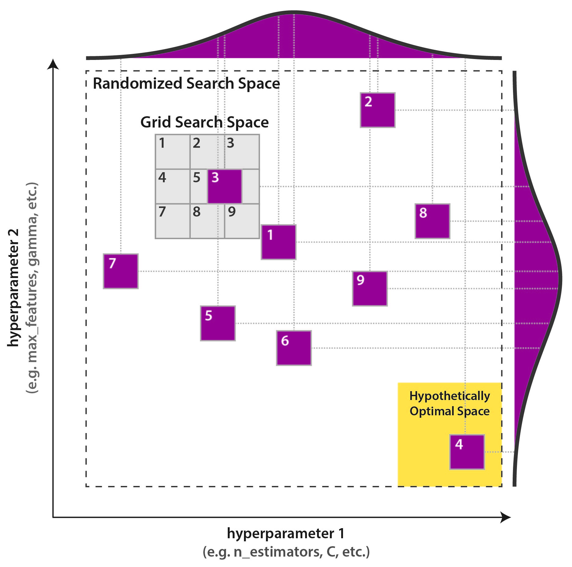
주요 장점 :
- 의미없는 매개 변수에 시간을 소비하지 앉음. 모든 단계에서 무작위 검색은 모든 매개 변수를 변경합니다.
- 평균적으로 그리드 검색보다 훨씬 빠르게 ~ 최적의 매개 변수를 찾습니다.
- 연속 매개 변수를 최적화 할 때 그리드에 의해 제한되지 않습니다.
단점:
- 그리드에서 글로벌 최적 매개 변수를 찾지 못할 수 있습니다.
- 모든 단계는 독립적입니다. 모든 특정 단계에서 지금까지 수집 된 결과에 대한 정보를 사용하지 않습니다.
예제는, sklearn.model_selection에서 RandomizedSearchCV를 사용합니다. 매우 넓은 매개 변수 공간으로 시작하여 50 개의 무작위 단계 만 만들 것입니다.
수행속도:
- (18 CPU- 162core) Wall time: 2.51 s
- AMD 2700x (1 CPU - 8Core) Wall time: 3.08 s
%%time
from sklearn.model_selection import RandomizedSearchCV
from scipy.stats import randint

param_grid_rand={'learning_rate': np.logspace(-5, 0, 100),
                 'max_depth':  randint(2,20),
                 'n_estimators': randint(100,2000),
                 'random_state': [random_state]}

rs=RandomizedSearchCV(model, param_grid_rand, n_iter = n_iter, scoring='neg_mean_squared_error',
                n_jobs=-1, cv=kf, verbose=False, random_state=random_state)

rs.fit(train_data, train_targets)

rs_test_score=mean_squared_error(test_targets, rs.predict(test_data))

print('===========================')
print("Best MSE = {:.3f} , when params {}".format(-rs.best_score_, rs.best_params_))
print('===========================')
===========================
Best MSE = 3200.402 , when params {'learning_rate': 0.0047508101621027985, 'max_depth': 19, 'n_estimators': 829, 'random_state': 42}
===========================
CPU times: user 1.16 s, sys: 25 ms, total: 1.19 s
Wall time: 3.15 s
결과는 GridSearchCV보다 낫습니다. 더 적은 시간을 소비하고 더 완전한 검색을했습니다. 시각화를 살펴 보겠습니다.
- random search의 모든 단계는 완전히 무작위입니다. 쓸모없는 매개 변수에 시간을 소비하지 않는 데 도움이되지만 여전히 첫 번째 단계에서 수집 된 정보를 사용하여 후자의 결과를 개선하지 않습니다.
rs_results_df=pd.DataFrame(np.transpose([-rs.cv_results_['mean_test_score'],
                                         rs.cv_results_['param_learning_rate'].data,
                                         rs.cv_results_['param_max_depth'].data,
                                         rs.cv_results_['param_n_estimators'].data]),
                           columns=['score', 'learning_rate', 'max_depth', 'n_estimators'])
rs_results_df.plot(subplots=True,figsize=(10, 10))
array([<matplotlib.axes._subplots.AxesSubplot object at 0x7fbdc6dfd4a8>,
       <matplotlib.axes._subplots.AxesSubplot object at 0x7fbdc6d44668>,
       <matplotlib.axes._subplots.AxesSubplot object at 0x7fbdc6d78630>,
       <matplotlib.axes._subplots.AxesSubplot object at 0x7fbdc6d2c630>],
      dtype=object)

3. HyperBand
Research Paper HyperBand
Abstract 발췌: 머신 러닝 알고리즘의 성능은 좋은 하이퍼 파라미터 집합을 식별하는 데 매우 중요합니다. 최근 접근 방식은 베이지안 최적화를 사용하여 구성을 적응 적으로 선택하지만 적응 형 리소스 할당 및 조기 중지를 통해 임의 검색 속도를 높이는 데 중점을 둡니다. 반복, 데이터 샘플 또는 기능과 같은 사전 정의 된 리소스가 무작위로 샘플링 된 구성에 할당되는 순수 탐색 비 확률 적 무한 무장 밴디트 문제로 하이퍼 파라미터 최적화를 공식화합니다. 이 프레임 워크에 대해 새로운 알고리즘 인 Hyperband를 도입하고 이론적 속성을 분석하여 몇 가지 바람직한 보장을 제공합니다. 또한, 하이퍼 파라미터 최적화 문제 모음에 대해 Hyperband를 인기있는 베이지안 최적화 방법과 비교합니다. Hyperband는 다양한 딥 러닝 및 커널 기반 학습 문제에 대해 경쟁 업체보다 훨씬 빠른 속도를 제공 할 수 있습니다. © 2018 Lisha Li, Kevin Jamieson, Giulia DeSalvo, Afshin Rostamizadeh 및 Ameet Talwalkar.

- Hyperband Search는 최적화 검색 속도에 중점을 둡니다.
- n개의 하이퍼파라미터 조합을 랜덤 샘플링.
- 전체 resource를 n개로 분할하고, 하이퍼 파라미터 조합에 각각 할당하여 학습
- 각 학습 프로세스는 일정 비율 이상의 상위 조합을 남기고 버림.
수행속도:
- (18 CPU- 162core) Wall time: 2.51 s
- AMD 2700x (1 CPU - 8Core) Wall time: 1.19 s
cloud자원을 사용하는 경우 분산 자원의 준비 시간이 상대적으로 긴것을 볼수 있었음.
!git clone https://github.com/thuijskens/scikit-hyperband.git 2>/dev/null 1>/dev/null
!cp -r scikit-hyperband/* .
!python setup.py install 2>/dev/null 1>/dev/null
%%time
from hyperband import HyperbandSearchCV

from scipy.stats import randint as sp_randint
from sklearn.preprocessing import LabelBinarizer


param_hyper_band={'learning_rate': np.logspace(-5, 0, 100),
                 'max_depth':  randint(2,20),
                 'n_estimators': randint(100,2000),
                 #'num_leaves' : randint(2,20),
                 'random_state': [random_state]
                 }


hb = HyperbandSearchCV(model, param_hyper_band, max_iter = n_iter, scoring='neg_mean_squared_error', resource_param='n_estimators', random_state=random_state)


#%time search.fit(new_training_data, y)
hb.fit(train_data, train_targets)


hb_test_score=mean_squared_error(test_targets, hb.predict(test_data))

print('===========================')
print("Best MSE = {:.3f} , when params {}".format(-hb.best_score_, hb.best_params_))
print('===========================')
===========================
Best MSE = 3431.685 , when params {'learning_rate': 0.13848863713938717, 'max_depth': 12, 'n_estimators': 16, 'random_state': 42}
===========================
CPU times: user 13.4 s, sys: 64 ms, total: 13.5 s
Wall time: 2.06 s
hb_results_df=pd.DataFrame(np.transpose([-hb.cv_results_['mean_test_score'],
                                         hb.cv_results_['param_learning_rate'].data,
                                         hb.cv_results_['param_max_depth'].data,
                                         hb.cv_results_['param_n_estimators'].data]),
                           columns=['score', 'learning_rate', 'max_depth', 'n_estimators'])
hb_results_df.plot(subplots=True,figsize=(10, 10))
array([<matplotlib.axes._subplots.AxesSubplot object at 0x7fbdc6c3f7f0>,
       <matplotlib.axes._subplots.AxesSubplot object at 0x7fbdc6c2a358>,
       <matplotlib.axes._subplots.AxesSubplot object at 0x7fbdc6bd4320>,
       <matplotlib.axes._subplots.AxesSubplot object at 0x7fbdc6b882b0>],
      dtype=object)

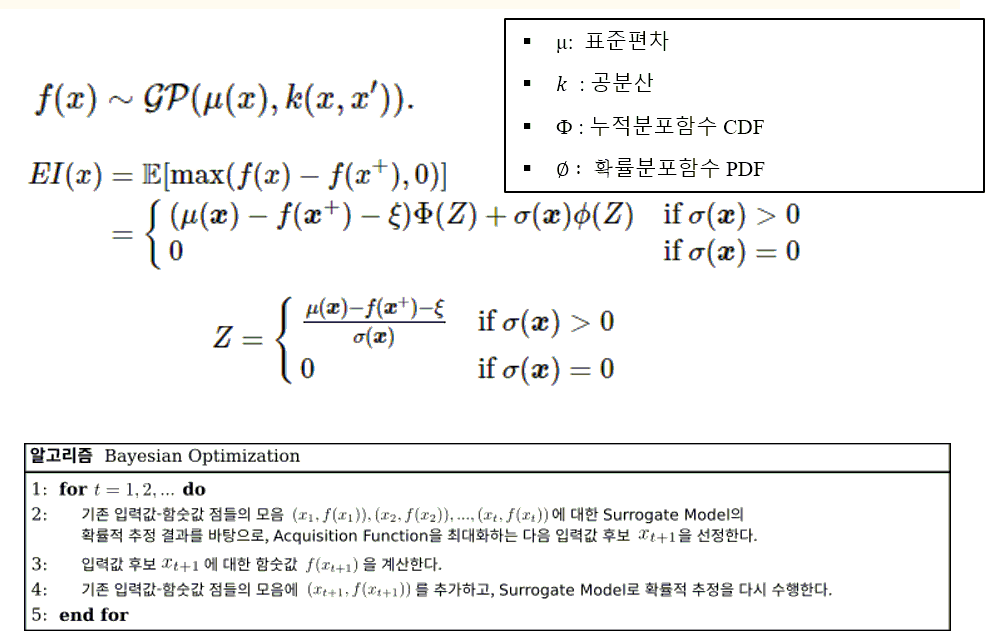
4. Bayesian optimization
Research Paper Bayesian optimization
Random 또는 Grid Search와 달리 베이지안 접근 방식은 목표 함수의 점수 확률에 하이퍼 파라미터를 매핑하는 확률 모델을 형성하는데 사용하는 과거 평가 결과를 추적합니다.

P(Score | Hyperparameters)
논문에서 이 모델은 목적 함수에 대한 "surrogate"라고하며 p (y | x)로 표시됩니다. surrogate 함수는 목적 함수보다 최적화하기 훨씬 쉬우 며 베이지안 방법은 대리 함수에서 가장 잘 수행되는 하이퍼 파라미터를 선택하여 실제 목적 함수를 평가할 다음 하이퍼 파라미터 세트를 찾는 방식으로 작동합니다.
pseudo code로 정리하면:
- 목적 함수의 대리 확률 모델 구축
- surrogate에서 가장 잘 수행되는 하이퍼 파라미터를 찾습니다.
- 이러한 하이퍼 파라미터를 실제 목적 함수에 적용
- 새 결과를 통합하는 대리 모델 업데이트
- 최대 반복 또는 시간에 도달 할 때까지 2-4 단계를 반복합니다.
더 깊이있는 베이지안 최적화에 대한 훌륭한 커널은 여기 참조: https://www.kaggle.com/artgor/bayesian-optimization-for-robots
-
Surrogate Model : 현재까지 조사된 입력값-함숫값 점들 ${(𝑥_1,f(𝑥_1)), ..., (𝑥_𝑡,f(𝑥_𝑡))}$ 를 바탕으로, 미지의 목적 함수의 형태에 대한 확률적인 추정을 수행하는 모델
-
Acquisition Function: 목적 함수에 대한 현재까지의 확률적 추정 결과를 바탕으로, ‘최적 입력값 ${𝑥^∗}$를 찾는 데 있어 가장 유용할 만한’ 다음 입력값 후보 ${𝑥_(𝑡+1)}$을 추천해 주는 함수 Expected Improvement(EI) 함수를 사용한다.
수행속도:
- (18 CPU- 162core) Wall time: 2min 24s
- AMD 2700x (1 CPU - 8Core) Wall time: 1min 36s
상대적으로 로컬테스트의 수행 속도가 빠른것을 볼수있었다.
#! pip install scikit-optimize
#https://towardsdatascience.com/hyperparameter-optimization-with-scikit-learn-scikit-opt-and-keras-f13367f3e796
from skopt import BayesSearchCV
from skopt.space import Real, Categorical, Integer
%%time

search_space={'learning_rate': np.logspace(-5, 0, 100),
                 "max_depth": Integer(2, 20),
                 'n_estimators': Integer(100,2000),
                 'random_state': [random_state]}


def on_step(optim_result):
    """
    Callback meant to view scores after
    each iteration while performing Bayesian
    Optimization in Skopt"""
    score = bayes_search.best_score_
    print("best score: %s" % score)
    if score >= 0.98:
        print('Interrupting!')
        return True

bayes_search = BayesSearchCV(model, search_space, n_iter=n_iter, # specify how many iterations
                                    scoring='neg_mean_squared_error', n_jobs=-1, cv=5)
bayes_search.fit(train_data, train_targets, callback=on_step) # callback=on_step will print score after each iteration

bayes_test_score=mean_squared_error(test_targets, bayes_search.predict(test_data))

print('===========================')
print("Best MSE = {:.3f} , when params {}".format(-bayes_search.best_score_, bayes_search.best_params_))
print('===========================')
best score: -4415.920614880022
best score: -4415.920614880022
best score: -4415.920614880022
best score: -4415.920614880022
best score: -4116.905834420919
best score: -4116.905834420919
best score: -4116.905834420919
best score: -4116.905834420919
best score: -4116.905834420919
best score: -3540.855689828868
best score: -3467.4059934906645
best score: -3467.4059934906645
best score: -3467.4059934906645
best score: -3467.4059934906645
best score: -3467.4059934906645
best score: -3467.4059934906645
best score: -3467.4059934906645
best score: -3467.4059934906645
best score: -3467.4059934906645
best score: -3465.869585251784
best score: -3462.4668073239764
best score: -3462.4668073239764
best score: -3462.4668073239764
best score: -3460.603434822278
best score: -3460.603434822278
best score: -3460.603434822278
best score: -3460.603434822278
best score: -3460.603434822278
best score: -3460.603434822278
best score: -3460.603434822278
best score: -3460.603434822278
best score: -3459.5705953392157
best score: -3456.063877875675
best score: -3456.063877875675
best score: -3454.9987003394112
best score: -3454.9987003394112
best score: -3454.9987003394112
best score: -3454.9987003394112
best score: -3454.9987003394112
best score: -3454.9987003394112
best score: -3454.9987003394112
best score: -3454.9987003394112
best score: -3454.9987003394112
best score: -3454.9987003394112
best score: -3454.9987003394112
best score: -3454.9987003394112
best score: -3454.9987003394112
best score: -3454.9987003394112
best score: -3454.9987003394112
best score: -3454.9987003394112
===========================
Best MSE = 3454.999 , when params OrderedDict([('learning_rate', 0.005336699231206307), ('max_depth', 2), ('n_estimators', 655), ('random_state', 42)])
===========================
CPU times: user 1min 59s, sys: 3min 34s, total: 5min 33s
Wall time: 1min 26s
bayes_results_df=pd.DataFrame(np.transpose([
                                         -np.array(bayes_search.cv_results_['mean_test_score']),
                                         np.array(bayes_search.cv_results_['param_learning_rate']).data,
                                         np.array(bayes_search.cv_results_['param_max_depth']).data,
                                         np.array(bayes_search.cv_results_['param_n_estimators']).data
                                        ]),
                           columns=['score', 'learning_rate', 'max_depth', 'n_estimators'])


bayes_results_df.plot(subplots=True,figsize=(10, 10))
array([<matplotlib.axes._subplots.AxesSubplot object at 0x7fbd6bfcc208>,
       <matplotlib.axes._subplots.AxesSubplot object at 0x7fbd68640470>,
       <matplotlib.axes._subplots.AxesSubplot object at 0x7fbd686b97f0>,
       <matplotlib.axes._subplots.AxesSubplot object at 0x7fbd686f1c50>],
      dtype=object)

5.Hyperopt
- 이 알고리즘을 다루기 위해 hyperopt [https://github.com/hyperopt/hyperopt] 라이브러리를 사용합니다.
- 현재, 하이퍼 파라미터 최적화를위한 최신 라이브러리중 하나입니다.
#!pip install hyperopt
우선 hyperopt에서 몇 가지 유용한 함수를 소개합니다.
- fmin : 최소화 메인 목적 함수
- tpe and anneal : optimization 접근방식
- hp : 다양한 변수들의 분포 포함
- Trials : logging에 사용
from hyperopt import fmin, tpe, hp, anneal, Trials
hyperop.fmin의 인터페이스는 Grid 또는 Randomized search와 다릅니다. 먼저, 최소화 할 함수를 정의합니다.
- 아래는 'learning_rate', 'max_depth', 'n_estimators'와 같은 다양한 매개 변수를 최소화하는 gb_mse_cv () 함수가 있습니다.
def gb_mse_cv(params, random_state=random_state, cv=kf, X=train_data, y=train_targets):
    # the function gets a set of variable parameters in "param"
    params = {'n_estimators': int(params['n_estimators']),
              'max_depth': int(params['max_depth']),
             'learning_rate': params['learning_rate']}

    # we use this params to create a new LGBM Regressor
    model = LGBMRegressor(random_state=random_state, **params)

    # and then conduct the cross validation with the same folds as before
    score = -cross_val_score(model, X, y, cv=cv, scoring="neg_mean_squared_error", n_jobs=-1).mean()

    return score
5.1 Tree-structured Parzen Estimator(TPE)
Research Paper TPE
TPE는 Hyperopt의 기본 알고리즘입니다. 최적화를 위해 베이지안 접근 방식을 사용합니다. 모든 단계에서 함수의 확률 모델을 구축하고 다음 단계에서 가장 유망한 매개 변수를 선택하려고합니다. 일반적으로 이러한 유형의 알고리즘은 다음과 같이 작동합니다.
- 1.임의의 initial point 생성 ${x^*}$
- 2.${F(x^*)}$ 계산
- 3.trials 로깅 이력을 사용해서, 조건부 확률모델 $P(F | x)$를 생성
- 4.$ P (F | x) $에 따라 $ {F (x_i)} $가 더 나아질 가능성이 가장 높은 $ {x_i} $를 선택합니다.
- 5.$ {F (x_i)} $의 real values를 계산합니다.
- 6.중지 기준 중 하나가 충족 될 때까지 3-5 단계를 반복합니다 (예 : i> max_eval).
예를 들어 특정 TPE 알고리즘에 대한 자세한 정보는 아래 링크 참조. (이 링크 내용은 상세버전으로, 튜토리얼의 범위를 벗어납니다.)
[https://towardsdatascience.com/a-conceptual-explanation-of-bayesian-model-based-hyperparameter-optimization-for-machine-learning-b8172278050f]
- fmin의 사용은 매우 간단합니다. 매개 변수의 가능한 공간을 정의하고 함수를 호출하기 만하면됩니다.
수행속도:
- (18 CPU- 162core) Wall time: 7.3s
- AMD 2700x (1 CPU - 8Core) Wall time: 7.98s
%%time

# possible values of parameters
space={'n_estimators': hp.quniform('n_estimators', 100, 2000, 1),
       'max_depth' : hp.quniform('max_depth', 2, 20, 1),
       'learning_rate': hp.loguniform('learning_rate', -5, 0)
      }

# trials will contain logging information
trials = Trials()

best=fmin(fn=gb_mse_cv, # function to optimize
          space=space,
          algo=tpe.suggest, # optimization algorithm, hyperotp will select its parameters automatically
          max_evals=n_iter, # maximum number of iterations
          trials=trials, # logging
          rstate=np.random.RandomState(random_state) # fixing random state for the reproducibility
         )

# computing the score on the test set
model = LGBMRegressor(random_state=random_state, n_estimators=int(best['n_estimators']),
                      max_depth=int(best['max_depth']),learning_rate=best['learning_rate'])
model.fit(train_data,train_targets)
tpe_test_score=mean_squared_error(test_targets, model.predict(test_data))

print("Best MSE {:.3f} params {}".format( gb_mse_cv(best), best))
100%|██████████| 50/50 [00:06<00:00,  8.32trial/s, best loss: 3186.7910608402444]
Best MSE 3186.791 params {'learning_rate': 0.026975706032324936, 'max_depth': 20.0, 'n_estimators': 168.0}
CPU times: user 784 ms, sys: 37 ms, total: 821 ms
Wall time: 6.08 s
Best MSE 3186로 RandomizedSearch에 비해 시간은 걸리지만, 좀 더 나은 솔루션을 찾았습니다.
tpe_results=np.array([[x['result']['loss'],
                      x['misc']['vals']['learning_rate'][0],
                      x['misc']['vals']['max_depth'][0],
                      x['misc']['vals']['n_estimators'][0]] for x in trials.trials])

tpe_results_df=pd.DataFrame(tpe_results,
                           columns=['score', 'learning_rate', 'max_depth', 'n_estimators'])
tpe_results_df.plot(subplots=True,figsize=(10, 10))
array([<matplotlib.axes._subplots.AxesSubplot object at 0x7fbd5e386c88>,
       <matplotlib.axes._subplots.AxesSubplot object at 0x7fbd5e2f9828>,
       <matplotlib.axes._subplots.AxesSubplot object at 0x7fbd5e3f7828>,
       <matplotlib.axes._subplots.AxesSubplot object at 0x7fbd5e426c88>],
      dtype=object)

Results
모든 접근 방식에 대해 iterations 수에 따른 best_cumulative_score를 시각화 해봅니다.
scores_df=pd.DataFrame(index=range(n_iter))
scores_df['Grid Search']=gs_results_df['score'].cummin()
scores_df['Random Search']=rs_results_df['score'].cummin()
scores_df['Hyperband']=hb_results_df['score'].cummin()
scores_df['Bayesian optimization ']=bayes_results_df['score'].cummin()
scores_df['TPE']=tpe_results_df['score'].cummin()


ax = scores_df.plot()

ax.set_xlabel("number_of_iterations")
ax.set_ylabel("best_cumulative_score")
Text(0, 0.5, 'best_cumulative_score')

-
Random Search는 단순하면서, 시간의 비용에 따른 스코어가 높은 것을 알 수 있었습니다.
-
TPE 알고리즘은 실제로 이후 단계에서도 시간이 지남에 따라 검색 결과를 지속적으로 개선하는 반면, Random search는 처음에 상당히 좋은 솔루션을 무작위로 찾은 다음 결과를 약간만 개선했습니다.
-
TPE와 RandomizedSearch 결과의 현재 차이는 매우 작지만, 더 다양한 범위의 하이퍼 파라미터를 사용하는 일부 실제 애플리케이션에서 hyperopt는 상당한 시간 대비 점수 향상을 제공 할 수 있으리라 봅니다.
-
참고 : 실제 생활에서는 비교를 위해 여러 번 반복하지 않고 시간을 사용하는 것이 더 정확하지만 장난감 예제에서는 tpe 및 어닐링의 추가 계산에 소요되는 시간의 비율이 cross_val_score 계산 시간에 비해 높으므로 반복 횟수와 관련하여 하이퍼 옵트 및 플롯 점수의 계산 속도에 대해 오해하지 않기로 결정했습니다.
실제 Evaluate 테스트 데이터를 이용해 결과를 비교하고 교차 검증 결과와 inline 확인하겠습니다.
print('Test MSE scored:')
print("Grid Search : {:.3f}".format(gs_test_score))
print("Random Search :  {:.3f}".format(rs_test_score))
print("Hyperband : {:.3f}".format(hb_test_score))
print("Bayesian optimization : {:.3f}".format(bayes_test_score))
print("TPE : {:.3f}".format(tpe_test_score))
Test MSE scored:
Grid Search : 3045.329
Random Search :  2877.117
Hyperband : 2852.900
Bayesian optimization : 2710.621
TPE : 2942.574
Test data의 evaluation에서는 Bayesian optimization 알고리즘을 사용한 하이퍼파라미터의 모델 MSE 점수가 가장 낮은것으로 나타났습니다. (실험용 Toy dataset으로 실행에 따라 결과임을 참고)
- Accuinsight+의 modeler AutoDL에 적용한 다양한 하이퍼 파라미터 최적화 접근 방식에 대해 알아봤습니다.
- 최신 hyperopt의 TPE알고리즘의 사용방법을 알 수 있었습니다.
- 실제 모델링 환경에서는, 실제로 어떤 접근 방식이 가장 좋은지 미리 알 수 없으며, 때로는 간단한 RandomizedSearch가 좋은 선택이 될 수 있으므로 항상 알아두면 유용합니다.
- 이 튜토리얼이 향후 ML, DL 프로젝트에서 많은 시간을 절약하기를 바랍니다.