Create function to plot wind field of the storm at specific times along the storm's track

[geanders]

Let's see if we can make a function that will generate the wind field of the storm over one or more time points---for example, a set of panels that show the wind field as the storm makes landfall.

[geanders]

Here's the pdf vignette where we've got the code for that example: Details of stormwindmodel package (1).pdf

[geanders]

Here's some more on making vector fields in R with ggplot:

https://r-graphics.org/recipe-miscgraph-vectorfield

[geanders]

For mapping, we'll want to use simple features (with the sf package---it lets us do the mapping in a ggplot framework). Here's some on how to do that: https://geanders.github.io/RProgrammingForResearch/reporting-results-2.html#simple-features

[geanders]

It looks like there might be some interesting ideas on how to do this here, too: https://semba-blog.netlify.app/03/20/2019/plotting-streamlines-of-surface-current-with-ggplot2-and-metr-package/

This uses a package called metR that helps with tidy data approaches to meteorological data: https://github.com/eliocamp/metR

[geanders]

Here's another lead---a package with a new geom called geom_quiver: https://cran.r-project.org/web/packages/ggquiver/readme/README.html

[geanders]

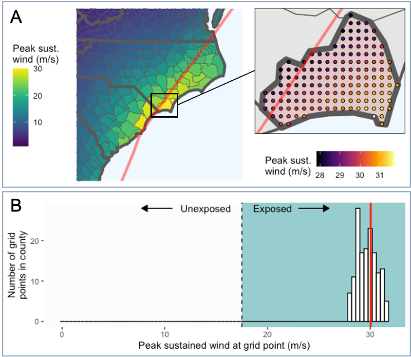
For making a grid, you can use st_make_grid. I've got some old code on this that I used to make this figure:

library(hurricaneexposuredata)
library(hurricaneexposure)
library(stormwindmodel)

library(tigris)
library(sf)
library(tidyverse)
library(viridis)
library(cowplot)
library(gridExtra)

data("hurr_tracks")
data("county_centers")
data("storm_winds")

example_state <- c("North Carolina", "South Carolina", 
                   "Virginia", "Georgia", "Tennessee", 
                   "Kentucky", "West Virginia")

example_storm <- "Charley-2004"
example_storm_track <- hurr_tracks %>% 
  filter(storm_id == example_storm)
example_storm_track_sf <- example_storm_track %>% 
  st_as_sf(coords = c("longitude", "latitude"), 
           crs = 4269) %>% 
  st_combine() %>% 
  sf::st_cast("LINESTRING")
example_storm_wind <- storm_winds %>% 
  filter(storm_id == example_storm)

study_states <- states(cb = TRUE, resolution = '20m') %>% 
  filter(NAME %in% example_state)
study_counties <- counties(state = example_state, 
                           cb = TRUE, resolution = "20m") %>% 
  mutate(fips = str_c(STATEFP, COUNTYFP)) %>% 
  left_join(example_storm_wind, by = "fips")

example_county_centers <- county_centers %>% 
  filter(state_name %in% example_state)

(a <- ggplot() + 
  geom_sf(data = study_counties, 
          aes(fill = vmax_sust, color = vmax_sust)) + 
  geom_sf(data = study_counties, fill = NA, size = 0.2) + 
  geom_sf(data = study_states, fill = NA, size = 1.5) + 
  geom_sf(data = example_storm_track_sf, color = "red", 
          size = 1.5, alpha = 0.5) + 
  # geom_rect(xmin = -78.65, xmax = -77.89, ymin = 33.85, ymax = 34.37, 
  #           fill = NA, colour = "black", size = 1) +
  xlim(-82, -75) + 
  ylim(31.5, 37.5) + 
  theme(panel.grid.major = element_blank(), 
        axis.text = element_blank(),
        axis.ticks = element_blank(),
        panel.background = element_rect(fill = "aliceblue"), legend.position = "left") +
  scale_fill_viridis(name = "Peak sust.\nwind (m/s)") + 
  scale_color_viridis(name = "Peak sust.\nwind (m/s)") )

ex_county_state <- "37"
ex_county_name <- "Brunswick"
example_county <- study_counties %>% 
  filter(STATEFP == ex_county_state, 
         NAME == ex_county_name) %>% 
  st_transform(6437) 

grid_spacing <- 4000
example_grid <- st_make_grid(example_county, square = TRUE, what = "centers",
                        cellsize = c(grid_spacing, grid_spacing)) %>% 
  st_sf() %>% 
  mutate(gridid = as.character(1:n()))

grid_to_model <- example_grid %>% 
  st_transform(4269) %>% 
  st_geometry() %>% 
  unlist() %>% 
  matrix(ncol = 2,byrow = TRUE) %>% 
  as_tibble() %>% 
  setNames(c("glon","glat")) %>% 
  mutate(gridid = as.character(1:n()),
         glandsea = TRUE) %>% 
  select(gridid, glat, glon, glandsea)

example_winds <- get_grid_winds(hurr_track = example_storm_track,
                                grid_df = grid_to_model)

example_grid <- example_grid %>% 
  left_join(example_winds, by = "gridid")

(b <- ggplot() + 
  #geom_sf(data = study_counties %>% st_transform(6437),
  #        aes(fill = vmax_sust, color = vmax_sust)) + 
  geom_sf(data = study_counties %>% st_transform(6437)) + 
  geom_sf(data = study_states%>% st_transform(6437), 
          fill = NA, size = 1.5) + 
  geom_sf(data = example_county, size = 3, 
          aes(fill = vmax_sust), alpha = 0.2) + 
  geom_sf(data = example_grid, shape = 21, 
          aes(fill = vmax_sust)) + 
  geom_sf(data = example_storm_track_sf, color = "red", 
          size = 1.5, alpha = 0.5) + 
  xlim(417173.7, 487643.9) + 
  ylim(1057597, 1116335) + 
  theme(panel.grid.major = element_blank(), 
        axis.text = element_blank(),
        axis.ticks = element_blank(),
        panel.border = element_rect(fill = NA),
        panel.background = element_rect(fill = "aliceblue"), legend.position = "left") +
  scale_fill_viridis(name = "Peak sust.\nwind (m/s)", 
                     option = "B") + 
  theme(legend.position = "bottom"))


(c <- ggplot(example_winds) + 
  geom_rect(xmin = -Inf, xmax = 17.5, 
            ymin = -Inf, ymax = Inf, 
            fill = "white", alpha = 0.2) + 
  geom_rect(xmin = 17.5, xmax = Inf, 
            ymin = -Inf, ymax = Inf, 
            fill = "paleturquoise3", alpha = 0.2) + 
  geom_histogram(aes(x = vmax_sust), binwidth = 0.4, 
                 fill = "white", color = "black") + 
  expand_limits(x = 0) + 
  geom_vline(xintercept = 17.5, linetype = 2) + 
  geom_vline(xintercept = example_county$vmax_sust, 
             color = "red", size = 1) + 
  annotate(geom = "text", x = 14, y = 28, 
           label = "Unexposed") + 
  annotate(geom = "text", x = 20.5, y = 28, 
           label = "Exposed") + 
  annotate("segment", 
           x = 23, xend = 26, 
           y = 28, yend = 28, 
           arrow = arrow(type = "closed", length = unit(0.1, "inches"))) + 
  annotate("segment", 
           x = 10.75, xend = 7.75, 
           y = 28, yend = 28, 
           arrow = arrow(type = "closed", length = unit(0.1, "inches"))) +
  labs(x = "Peak sustained wind at grid point (m/s)", 
       y = "Number of grid\npoints in county"))


g1 <- grid.arrange(grobs = list(a, b), 
                   layout_matrix = rbind(c(1, 1, 1, NA, NA),
                                         c(1, 1, 1, 2, 2),
                                         c(1, 1, 1, 2, 2),
                                         c(1, 1, 1, 2, 2),
                                         c(1, 1, 1, NA, NA)))

grid.arrange(grobs = list(g1, c), 
             layout_matrix = rbind(c(1, 1),
                                   c(1, 1),
                                   c(2, 2)))