Implementing eigenspace beamformer lcmv
Implementing the eigenspace beamformer from the paper:
Sekihara K, Nagarajan SS, Poeppel D, Marantz A, Miyashita Y (2002) Application of an MEG eigenspace beamformer to reconstructing spatio-temporal activities of neural sources. Human Brain Mapping 15:199–215.
It seems this was begun at one point but not finished using the undocumented subspace field. I have done my implementation independently of the subspace field. I can remove or change the subspace option as deemed necessary.
Let me know if you want more explicit references to the paper by adding comments and so
Hi Lau, I am pretty sure that the subspace argument (in case it's single number >=1) is doing exactly what you intend to do.
Indeed, the subspace is undocumented, and a bit fuzzy (I implemented it a long time ago, and haven't used it extensively since -> note that I am familiar with Kensuke's formulation and I ensured back then that the current implementation behaves very similar, pity I did not document this better). Right now, if I recall well, with subspace, you can do 3 things:
- it's a single positive number < 1, in which case the svd-spectrum of the Covariance is truncated in order to select the number of components to be kept for the eigenspace projection
- it's a single positive number > 1, in which case the Sekihara like eigenspace beamformer is computed.
- it's a matrix (which could also allow for for the prewhitening beamformer for instance (as per one of Kensuke's other papers), although these days there is the possibility to prewhiten the data with ft_denoise_prewhiten, and subsequently one could use the prewhitened grad array, in combination with the prewhitened data to beamform in whitened space. As a matter of fact, something very similar (in equivalence to the eigenspace beamformer) should be possible with doing ft_componentanalysis (with 'pca'), and then compute leadfields with comp.grad + beamform the components.
For each of the cases the data and the leadfields are projected into the subspace, and the spatial filter is computed using the normal beamformer formulas. This, as far as I remember, is equivalent to Kensuke's formulations.
I am reluctant to accept the current suggestions, because it treats the eigenspace as a special case (which it isn't), generating new sets of variables (Gamma, mu, etc -> bad for code readability and maintainability), and because it implements something which can most likely already be more or less achieved with the current code. As a side note, lf can be a matrix still (i.e. there is no guarantee that the user specifies 'fixedori', nor a prerequisite, so the current definition of 'mu' does not work for vector formulations.
Could you verify the extent to which your implementation behaves very different from the current one? I think that is relatively straightforward, either use 'eigenspace', <X>, or 'subspace', <X> as key-value pairs.
Hi Jan-Mathijs
Thanks for going over it! I appreciate your points about treating it as a special case and introducing new variables. The reason for my implementing it all over is that it was hard for me to parse the subspace method. It does also provide different results. Here it is tested on the data from here: https://www.fieldtriptoolbox.org/tutorial/beamformer_lcmv/
These are the calls
cfg                  = [];
cfg.method           = 'lcmv';
cfg.sourcemodel      = lf; % leadfield
cfg.headmodel        = headmodel; % volume conduction model (headmodel)
cfg.lcmv.keepfilter  = 'yes';
cfg.lcmv.fixedori    = 'yes'; % project on axis of most variance using SVD
cfg.lcmv.weightnorm  = 'arraygain';
cfg.lcmv.eigenspace  = 'no';

source               = ft_sourceanalysis(cfg, timelock);

cfg.lcmv.eigenspace  = Q;

source_eigenspace    = ft_sourceanalysis(cfg, timelock);

cfg.lcmv.eigenspace  = 'no';
cfg.lcmv.subspace    = Q;

source_subspace      = ft_sourceanalysis(cfg, timelock);
Let me know if you want a fully reproducible script! I will also go check my implementations of the equations again. I've updated allowing for the prewhitening, but I do not intend for that part to be pulled. Looking forward to hearing what you think
Nice! thanks for taking up the challenge. Would it be a big deal to upload the script as a 'test' function in fieldtrip/test?
I'll take up the challenge You'll hear from me when I have implemented the test
Well you could also just dump the script you have so far, and then we'll work on it together a bit.
OK, thanks. I will in the meantime work a bit overall on cleaning up the tutorial that you managed to find. It has never been broadcasted/linked from the main tutorial index page, and it seems that not much is needed for that.
If OK with you, I'll push a test/test_tutorial_beamformer_lcmv into this branch, which will then also force me to constructively get your efforts implemented into the codebase ...
BTW, I chatted about this a bit with @robertoostenveld and we indeed realised that some early code design decisions, in combination with the fact that many of the BF-variants have mathematical-implementational details that make it challenging to easily accommodate in the current code structure. One the one hand there is scientific transparency, which ideally has a one-to-one mapping between some acronymal method descirbed in a paper, and an m-file that does the exact implementation according to the formulas in the referenced paper. On the other hand (mostly the current situation) there are code efficiency (and prospective code maintainability issues) that have led to the now somewhat opaque code structure here and there.
As a possible development we could consider the model that currently exists for the SAM beamformer, which has its own m-file. So, in other words, we may discuss the 'bestaansrecht' of a separate ft_inverse_beamformer_eigenspace or so, that is mapped directly onto the formulation in Kensuke's paper.
On the other hand I'd be still very interested in checking out the different implementation, and understand why they yield different results.
Fine that you pushed the test in here I understand the tension between having smooth code and having transparency. If deemed valuable, I would be happy contributing to an ft_inverse_beamformer_eigenspace For now, I have pushed the test script test/test_pull1773.m Have a look at it!
Hi Lau, I went through your test script, converted it into a function, made some changes, and importantly fixed an error in your implementation of the eigenspace BF (the use of rot90 was not correct). This makes both implementations relatively well aligned, although not identical. I agree with you that your implementation follows Sekihara's equations, but what's strange about that implementation is that the basic constraint w * l is not equal to the identity matrix (which is the basic constraint that the unit gain beamformer should fulfill -> not sure about whether this should be a requirement for the eigenspace BF as well). I will think about this a little bit more.
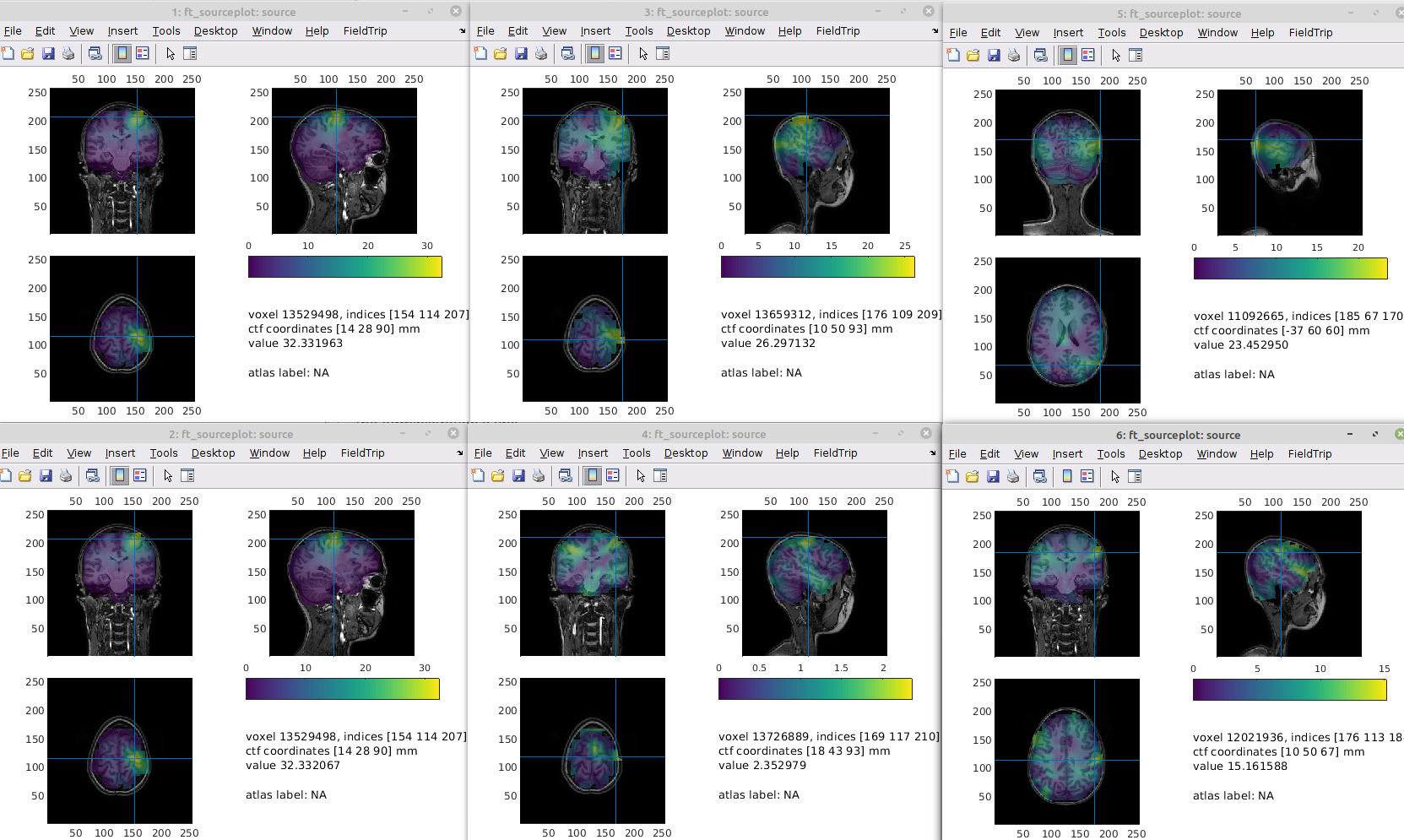
Hi Jan-Mathijs Very good you fixed the rotation error - I guess it just confirms what I heard at LiveMEEG - that you should have more eyes on your code. I remember you had that note (w * lf ~= I) in your original code as well... For a low number of components (10), it seems to make a big difference to the subspace implementation
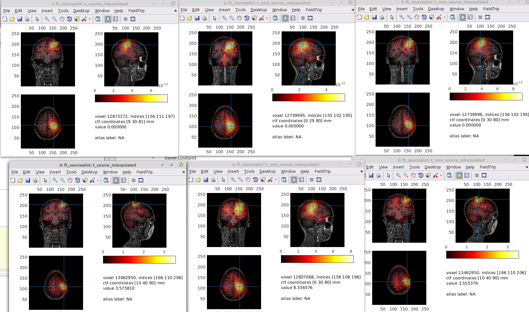
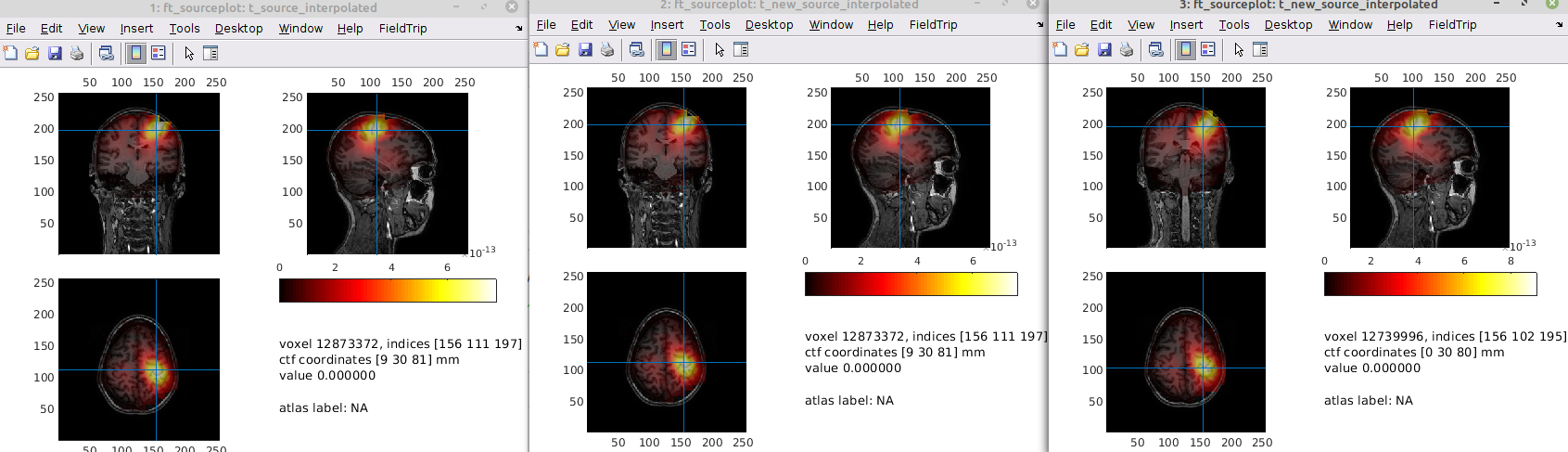
 source, source_eigenspace and source_subspace plotted in that order
Q = 10;

% create spatial filter using the lcmv beamformer
cfg                  = [];
cfg.method           = 'lcmv';
cfg.sourcemodel      = lf; % leadfield
cfg.headmodel        = headmodel; % volume conduction model (headmodel)
cfg.lcmv.keepfilter  = 'yes';
cfg.lcmv.fixedori    = 'yes'; % project on axis of most variance using SVD
cfg.lcmv.weightnorm  = 'arraygain';
cfg.lcmv.eigenspace  = 'no';

source               = ft_sourceanalysis(cfg, timelock);

cfg.lcmv.eigenspace  = Q;
cfg.lcmv.prewhitened = 'no';

source_eigenspace    = ft_sourceanalysis(cfg, timelock);

cfg.lcmv.eigenspace  = 'no';
cfg.lcmv.subspace    = Q;

source_subspace      = ft_sourceanalysis(cfg, timelock);
For a high number (76), it makes very little difference
what parameter are you plotting in the figures? Is it the 'mom' at a certain latency? Note that I have fooled around a bit with your definition (as well as with the weight normalisation settings for the source reconstruction -> basically no weightnorm for comparability) of what was to be plotted.
Yes, mom at 46 ms with arraygain - I understand that it is easier to use the unitgain to not complicate the matters too much - but it is hard to make sense of the unitgain plots without contrasting due to the central bias Furthermore, the source analyses on the prewhitened data look a bit weird now, but let's look at that later
but the prewhitening problem might be due to me not adapting the leadfield thanks for pointing that out! testing the plots I will get with the test function now
You might need to switch on the fixedori again (I switched it off for testing purposes, and probably committed that version)
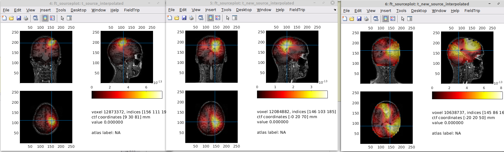
Here's plotting your implementation (with fixori) ("normal on top and whitened below) row: normal, eigenspace, subspace
 They also differ here
I suspect that there might be something off w.r.t. the optimal orientation estimate for the projection based BFs. Not sure, though.
hmm, with the array gain, they looked nice enough..., but could be worth looking into
Well, that's a good point, but also indicates that indeed it might be due to the orientation estimate: the arraygain uses a different heuristic to estimate the optimal orientation than the unit gain (cf. lines 342 vs. 356)... the normalisation of the leadfield is subsequently just a scalar normalisation, and should not affect the 'shape' of the spatial filter (thus only affects the scaling of the source time courses)
As a side note: I am now wondering about the 'fixedori' option in the beamformer functions, and its current fuzzy interaction with the different weightnorm options. I am aware of the fact that most of this derives from the equations presented in the Sekihara book, but I am not sure whether it is required to constrain the possible combinations of weightnorm/fixedori heuristics in the way it is currently constrained.
In other words, why don't we in principle support an NxM table of combinations of fixedori heuristics versus weightnorm options? Pinging @robertoostenveld and @britta-wstnr in case they want to chime in...
@schoffelen I would assume that you have to restrict the combinations if you want to maximize power through fixedori ...
Hi Lau @ualsbombe, what shall we do with this PR? I have added a snippet of code at the beginning of test_pull1573, which - at a low-level - compares the two implementations, i.e. the one you made that follows Kensuke's formulas, and the one that was already in FT (using a scalar number for the subspace argument). As I typed in the comment there, it seems that both implementations (in its scalar application, i.e. with a fixed leadfield orientation) yield up to a scaling the same filter weights. Things start to diverge in the vector case, and in the 'fixedori' case. For the latter, this is the consequence of the fact that different 'optimal' orientations are estimated. The vector case in 'your' implementation has a to me clearly undesired property of yielding a non-diagonal gain matrix (i.e. when filt * lf is computed).
Anyway, long story short, the differences observed in the downstream part of the test function are the consequence of the heuristic by which the optimal orientation is computed, and thus not necessarily the consequence of the difference in the 'core' implementation.
In the original publication I could not find anything back about the estimation strategy for getting the optimal orientation, nor was the paper very explicit about a vector version of the eigenspace beamformer. Therefore, I'd be inclined to not merge this PR (or perhaps only the first chunk of the test function). Part of which is also inspired by the fact that by now, some of the changes contain conflicts with the main branch, which need to be looked into etc.
What do you think? Also pinging @britta-wstnr in case she wants to chime in (but don't feel obliged).
Hmm, must admit I haven't thought about it for a while. So in their following book: Sekihara, K., Nagarajan, S.S., 2008. Adaptive Spatial Filters for Electromagnetic Brain Imaging. Springer Science & Business Media.
They have a chapter where they write "The eigenspace projection can also be applied to the vector formulation with no modification" (section 6.8.2). (I have a copy of the book I can share). I can't seem to find how they find the optimal orientation for the eigenspace scalar version though.
In terms of what to do with this pull request, I will talk with the other people in the project, hopefully Friday, and then I'll give you an update as to whether they have any insights.
To be honest, section 6.8.2 is not the strongest (and most easy to understand) section of the book. And that's even without consideration of the typos in equations 6.88-6.90...
I agree completely - that's why I based the implementation on the paper instead...
Sorry for the long silence - I have a meeting with the one who is actually using the implementation on Thursday - okay if I return with a status then? I suspect we can close it, but I just wanted to double-check with him, if he is still in need of it.
So during today's meeting, we saw quite some differences in the solutions that the eigenspace beamformer (my implementation) would come up with compared to the subspace implementation, where the eigenspace beamformer fared a lot better (sorry for the imprecise language). It's still very much work in progress, but we do believe that it fares better than the subspace implementation. @TamasMinarik is doing most of the testing on it these days, so I am pinging him here
That being said, it's of course fine closing the issue, until we are ready with a version that fits better into the FieldTrip way of doing things, and until we find the time backing up our bold claims. We can always return later with a new pull request ;-)