tectonics.js
 tectonics.js copied to clipboard
Precip/Evap Model Research
Found this while trying to find support for my k1 + k2cos(6lat) + k3(1-lat/90) - k4dist_to_cont_edge*sin(lat) model.
Evaporation and precipitation vs. latitude. http://www.roperld.com/science/Evaporation_PrecipitationVSLatitude.htm
This might prove useful…
Along the same vein, P-E might be a better input to the NPPp element of the Miami model, although that would require different coefficients on the curve fit to existing net primary production data.
We should be able to easily work that into the shader code - relevant code is in "scripts/view/fragment/template.glsl.c" and "scripts/view/fragment/FragmentShaders.js"
Something relevant to mention: for the last year or so I've been working on a experimental branch to overhaul the crust model to address problems while working on issue #8 and #1 (it's the "tests/field" branch if you want to try it out on your machine, if so let me know what you think). If I can get it working, it throws the door wide open for proper climate modeling. So now is a good time to think about pie-in-the-sky climate models, because they just might be feasible soon.
There's maybe just one issue I need to work out before I'm comfortable merging that branch with master. It needs to handle plate collision a bit more sensibly: continental docking, accretion, etc. It already generates sensible looking planets, but it doesn't have code in place to accrete continental crust, and I'm unsatisfied with that
useful or interesting links:
Rules of Thumb: http://web.archive.org/web/20130619132254/http://jc.tech-galaxy.com/bricka/climate_cookbook.html https://imgur.com/a/UNvLF#vrrcARn http://www.physicalgeography.net/fundamentals/7p.html
Navier stokes: http://www-users.cs.umn.edu/~narain/files/fluids2.pdf http://developer.download.nvidia.com/books/HTML/gpugems/gpugems_ch38.html http://jamie-wong.com/2016/08/05/webgl-fluid-simulation/ <-- this is the one where it finally clicked for me
also bought a super cheap book on amazon: https://books.google.com/books?id=3lcnDwAAQBAJ&printsec=frontcover#v=onepage&q=GCM&f=false. The 2nd edition is just $8
var FluidMechanics = {};

FluidMechanics.get_advected_ids = function (velocity, timestep, result, scratch) {
    var past_pos = scratch || VectorRaster(velocity.grid);
    var result   = result  || Uint16Raster(velocity.grid);
    VectorField.add_scalar_term (velocity.grid.pos, velocity, -timestep,    past_pos);
    VectorField.normalize(past_pos, past_pos);
    velocity.grid.getNearestIds    (past_pos,                                  result);
    return result;
}
// get pressure of an advected fluid
// An advected fluid has regions where fluid is compressed,
// but fluid simulation usually assumes fluid is incompressible.
// This method takes an advected fluid velocity, and
// isolates the "compressing" component from the "swirling" component.
// The "swirling" component is declared to be the actual fluid velocity.
// The "compressing" component is declared to be the pressure gradient.
// We use something called "Jacobi iteration" to isolate the two components.
// For more info: http://jamie-wong.com/2016/08/05/webgl-fluid-simulation/
FluidMechanics.refine_pressure_estimate = function (advected_velocity, pressure, result) {
  result = result || Float32Raster(grid);
  VectorField.divergence(advected_velocity, result);

  //TODO: need density and timestep somewhere here
  var neighbor_count = grid.neighbor_count;
  var average_differential = grid.average_differential * grid.average_differential;
  for (var i = 0; i < result.length; i++) {
  	result[i] *= -density;
  	result[i] /= timestep;
  	result[i] /= 4;
  	result[i] *= neighbor_count[i] * average_differential;
  }

  var arrows = field.grid.arrows;
  var arrow;
  for (var i=0, li=arrows.length; i<li; ++i) {
      arrow = arrows[i];
      result[arrow[0]] += pressure[arrow[1]] ;
  }
  for (var i = 0; i < result.length; i++) {
  	result[i] /= 4;
  }
  return result;
}

FluidMechanics.simulate = function(velocity, pressure, timestep, iterations, scratch_f32, scratch_ui8, scratch_vec) {
	// Step 1, advect velocity:
    var advected_velocity = scratch_f32;
	FluidMechanics.advect 	(velocity, velocity, timestep, scratch_ui8, 	advected_velocity)
	// copy so we can free up scratch_f32
	Float32Raster.copy 		(advected_velocity, velocity);

	// Step 2, find pressure:
	var temp = pressure;
	var refined_pressure = scratch_f32;
	for (var i = 0; i < iterations; i++) {
		FluidMechanics.refine_pressure_estimate(advected_velocity, pressure, refined_pressure);
		temp = pressure;
		pressure = refined_pressure;
		refined_pressure = temp;
	}
	// copy so we can free up scratch_f32
	Float32Raster.copy 		(pressure, refined_pressure);

	// Step 3, find velocity
    var pressure_gradient = scratch_vec;
    ScalarField.gradient 	(pressure, 										pressure_gradient);
	VectorRaster.sub_field	(velocity, pressure_gradient, 					velocity);

	return velocity;
}
OK, really excited now.
I'm prototyping a climate model based on what I see here: https://imgur.com/a/UNvLF#vrrcARn. Nowhere near scientifically valid (at least not yet), and probably has lots of bugs.
We start with a simple model for air pressure based on latitude. It's just a few bands of alternating high and low pressure, represented by cosine of latitude:
AtmosphericModeling.surface_air_pressure_lat_effect = function (lat, pressure) {
	pressure = pressure || Float32Raster(lat.grid);
	var cos = Math.cos;
	for (var i=0, li=lat.length; i<li; ++i) {
	    pressure[i] = -cos(5*(lat[i]));
	}
	return pressure
}
view.setScalarDisplay(new ScalarHeatDisplay( { min: '-1.', max: '1.',
		getField: function (world, effect, scratch) {
			var axial_tilt = Math.PI*23.5/180;
			var lat = Float32SphereRaster.latitude(world.grid.pos.y);
			AtmosphericModeling.surface_air_pressure_lat_effect(lat, effect);
			return effect;
		}
	} ));
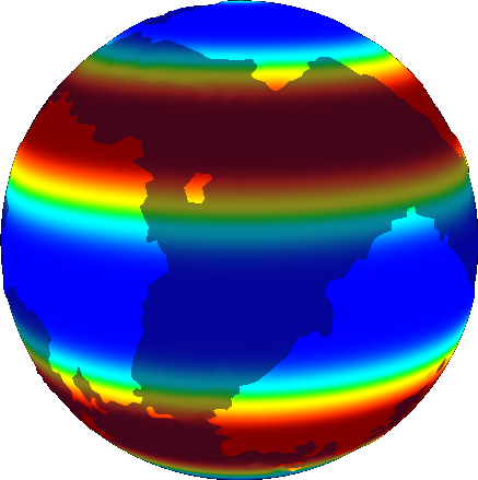
Offset the latitude to simulate winter (I think this is the right thing to do):
view.setScalarDisplay(new ScalarHeatDisplay( { min: '-1.', max: '1.',
		getField: function (world, effect, scratch) {
			var axial_tilt = Math.PI*23.5/180;
			var lat = Float32SphereRaster.latitude(world.grid.pos.y);
			var effective_lat = ScalarField.add_scalar(lat, axial_tilt);
			Float32RasterInterpolation.clamp(effective_lat, -Math.PI/2, Math.PI/2, effective_lat);
			AtmosphericModeling.surface_air_pressure_lat_effect(effective_lat, effect);
			return effect;
		}
	} ));

Result looks boring because there's no land. So let's find out where the land is:
view.setScalarDisplay(new ScalarHeatDisplay( { min: '-1.', max: '1.',
		getField: function (world, effect, scratch) {
			var lat = Float32SphereRaster.latitude(world.grid.pos.y);
			var is_land = ScalarField.gt_scalar(world.displacement, world.SEALEVEL);
			return is_land;
		}
	} ));
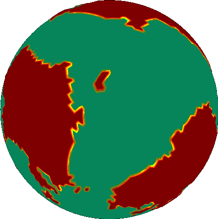
Smooth it out with binary morphology and the diffusion equation. This part is costly, performance-wise.
view.setScalarDisplay(new ScalarHeatDisplay( { min: '-1.', max: '1.',
		getField: function (world, effect, scratch) {
			var lat = Float32SphereRaster.latitude(world.grid.pos.y);
			var is_land = ScalarField.gt_scalar(world.displacement, world.SEALEVEL);
			BinaryMorphology.erosion(is_land, 2, is_land);
			Float32Raster.FromUint8Raster(is_land, effect);
			var diffuse = ScalarField.diffusion_by_constant;
			var smoothing_iterations =  2;
			for (var i=0; i<smoothing_iterations; ++i) {
				diffuse(effect, 1, effect, scratch);
			}
			return effect;
		}
	} ));

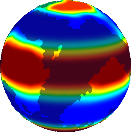
Land has different pressure effects depending on hemisphere. IIRC land in winter gets higher pressure:
view.setScalarDisplay(new ScalarHeatDisplay( { min: '-1.', max: '1.',
		getField: function (world, effect, scratch) {
			var lat = Float32SphereRaster.latitude(world.grid.pos.y);
			var is_land = ScalarField.gt_scalar(world.displacement, world.SEALEVEL);
			BinaryMorphology.erosion(is_land, 2, is_land);
			Float32Raster.FromUint8Raster(is_land, effect);
			var diffuse = ScalarField.diffusion_by_constant;
			var smoothing_iterations =  2;
			for (var i=0; i<smoothing_iterations; ++i) {
				diffuse(effect, 1, effect, scratch);
			}
			var pos = world.grid.pos;
			ScalarField.mult_field(effect, lat, effect);
			return effect;
		}
	} ));

Turn this into a function in the AtmosphericModeling namespace, and add a "season" parameter (season==1 for winter in the northern hemisphere and season==-1 for summer in the northern hemisphere)
AtmosphericModeling.surface_air_pressure_land_effect = function(displacement, lat, sealevel, season, effect, scratch) {
	var is_land = ScalarField.gt_scalar(displacement, sealevel);
	BinaryMorphology.erosion(is_land, 2, is_land);
	Float32Raster.FromUint8Raster(is_land, effect);
	var diffuse = ScalarField.diffusion_by_constant;
	var smoothing_iterations =  2;
	for (var i=0; i<smoothing_iterations; ++i) {
		diffuse(effect, 1, effect, scratch);
	}
	var pos = world.grid.pos;
	ScalarField.mult_field(effect, lat, effect);
    ScalarField.mult_scalar(effect, season, effect);
	return effect;
}
OK, now we add the two effects together:
AtmosphericModeling.surface_air_pressure = function(displacement, lat, sealevel, season, axial_tilt, pressure, scratch) {
	scratch = scratch || Float32Raster(lat.grid);
	// "effective latitude" is what the latitude is like weather-wise, when taking axial tilt into account
	var effective_lat = scratch;
	ScalarField.add_scalar(lat, season*axial_tilt, effective_lat);
	Float32RasterInterpolation.clamp(effective_lat, -Math.PI/2, Math.PI/2, effective_lat);

	AtmosphericModeling.surface_air_pressure_lat_effect(effective_lat, pressure);

	var land_effect = Float32Raster(lat.grid);
	var scratch2 = Float32Raster(lat.grid);
	AtmosphericModeling.surface_air_pressure_land_effect(displacement, effective_lat, sealevel, season, land_effect, scratch2);
	ScalarField.add_scalar_term(pressure, land_effect, 1, pressure);

	return pressure;
}
Density times the gradient of pressure is acceleration, but we pretend it's velocity.
view.setVectorDisplay( new VectorFieldDisplay( {
		getField: function (world) {
			var lat = Float32SphereRaster.latitude(world.grid.pos.y);
			var scratch = Float32Raster(world.grid);
			var pressure = Float32Raster(world.grid);
			AtmosphericModeling.surface_air_pressure(world.displacement, lat, world.SEALEVEL, 1, Math.PI*23.5/180, pressure, scratch);
			var velocity = ScalarField.gradient(pressure);
			return velocity;
		}
	} ));

Now just add the coriolis effect:
AtmosphericModeling.surface_air_velocity_coriolis_effect = function(pos, velocity, angular_speed, effect) {
	effect = effect || VectorRaster(pos.grid);
	VectorField.cross_vector_field	(velocity, pos, 			effect);
	VectorField.mult_scalar 		(effect, 2 * angular_speed, effect);
	VectorField.mult_scalar_field	(effect, pos.y, 			effect);
	return effect;
}
view.setVectorDisplay( new VectorFieldDisplay( {
		getField: function (world) {
			var lat = Float32SphereRaster.latitude(world.grid.pos.y);
			var scratch = Float32Raster(world.grid);
			var pressure = Float32Raster(world.grid);
			AtmosphericModeling.surface_air_pressure(world.displacement, lat, world.SEALEVEL, 1, Math.PI*23.5/180, pressure, scratch);
			var velocity = ScalarField.gradient(pressure);
			var coriolis_effect = AtmosphericModeling.surface_air_velocity_coriolis_effect(world.grid.pos, velocity, ANGULAR_SPEED)
			VectorField.add_vector_field(velocity, coriolis_effect, velocity);
			return velocity;
		}
	} ));
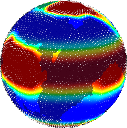
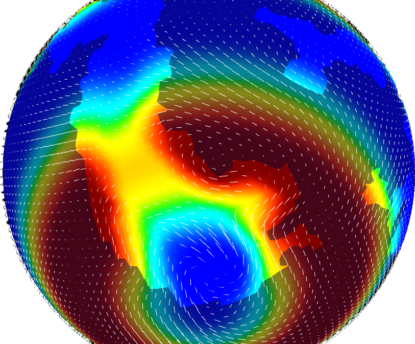
You can see how air gets deflected around landmass:
BTW, you should be able to run all this code in the Developer Tools console. I've also got a "atmo-model" branch out with this stuff added.
I have these features implemented in prod.
The models aren't strictly rigorous, not scientifically. Pressure and velocity are scaled to the right units, but the pressure model is hand wavey (kind of like existing models for precip and temp), and using gradients to find velocity is not strictly correct. Strictly, density times the gradient of pressure ought to be acceleration, not velocity, but it is suggestive of velocity and it's much more performant than actual fluid simulation.
I need a model that can be run in less than a single frame. It needs to return the average climate over millions of years, not years or decades. There's not a lot of GCMs that meet that criteria. I expect the correct model I'm looking for either relies on statistical mechanics or a steady state assumption. I need to do some more reading.
The next thing I'm going to work on is probably temperature. I have a branch out there to model orbital mechanics, specifically distance and orientation relative to the sun. I'd sample over several points in the day and several points in the year, find equilibrium temperature for a black body at each point, then average them out to get summer/winter temperature.
I'm going to have to look at this more closely later, but the pressure doesn't seem to take landmasses into account currently. I'm also just guessing here, but it looks like you're still using "my" handwavey precip model. Looking forward to a flow-based model.
In the longer run, it looks like that flow-based model may be applicable to overland water flow and thus considerably prettier erosion, and sediment deposition effects. If you get to that point, exporting high dynamic-range elevations will become a lot more urgent…😳😁😏
On Nov 11, 2017, at 4:04 PM, Carl Davidson [email protected] wrote:
I have these features implemented in prod.
The models aren't strictly rigorous, not scientifically. Pressure and velocity are scaled to the right units, but the pressure model is hand wavey (kind of like existing models for precip and temp), and using gradients to find velocity is not strictly correct. Strictly, the gradient of pressure ought to be acceleration, not velocity, but it is suggestive of velocity and it's much more performant than actual fluid simulation.
I need a model that can be run in less than a single frame. It needs to return the average climate over millions of years, not years or decades. There's not a lot of GCMs that meet that criteria. I expect the correct model I'm looking for either relies on statistical mechanics or a steady state assumption. I need to do some more reading.
The next thing I'm going to work on is probably temperature. I have a branch out there to model orbital mechanics, specifically distance and orientation relative to the sun. I'd sample over several points in the day and several points in the year, find equilibrium temperature for a black body, then average them out to get summer/winter temperature.
— You are receiving this because you authored the thread. Reply to this email directly, view it on GitHub, or mute the thread.
Pressure does take landmass into account, but the effect only exists during the solstices. Try moving the season slider.
Precip is still your model. I'm unsure how to continue on that front. I know high pressure regions like the "horse" latitudes should be drier. We could also advect wind velocity to determine where water evaporates from the ocean or where rain shadows exist. I don't have a good mechanistic model for evaporation or precipitation, but that's what I want as well.
Erosion is already flow based, in a way. It's sort of related to the gradient of elevation. I spent a lot of time thinking about ways to simulate river valleys this year though and it will take a different approach to do so. A problem I foresee will be grid resolution. It's already working close to the limits to what we can do in a single frame. We can speed up diffused pressure fields for the mantle and atmosphere by switching to a coarser grid, but we can't take that approach for river valleys.
EDIT: I misunderstood what you meant by flow based erosion. Yeah, any improvements we make to precipitation can be fed immediately into our erosion model.
Okay. I see the season slider now. As a preliminary model, it's very cool. It doesn't look like you have an arctic/antarctic high pressure zone. It's going to be strong, because the flow geometry and the really cold temperatures are going to collaborate to pile up low altitude air. My precip model is actually probably a better model for surface pressure(lows for high precip, highs for low precip, so an inverse model. It needs more research than I bothered with. It was definitely a bit of educated handwavery.
For a precip model. I think I might look into a "fetch"-based model. Trace winds back to the nearest patch of ocean and base precipitation on inverse distance traversed. The farther water is along the wind path, the less rain you get. Give bonuses for orographic uplift and penalties for falling terrain. Should work better than decreasing rainfall with distance from shoreline…
I also think the weaknesses in the temperature model start to make themselves apparent with that season slider. What it really is is an insolation model pretending to be a temperature model, much as pressure gradient is acceleration masquerading as velocity. Unfortunately, the downsides of that pretense show up a lot more clearly with the temperature model. If you are familiar with octave/matlab code, I can send you a decent-ish 1d+time insolation model and try to work up from that. May or may not be helpful.
As to eroding river valleys, that's a tough one. Even on an 8192x4096 equirectangular grid(I call that 8k), each pixel near the equator is going to represent something like 5km on the planetary surface. Also, to work decently, those river valleys are going to need to be at least 3 pixels wide minimum. Maybe 2 at the outside. Even a 16 or 32k equi grid is going to have a hell of a time with that, and realistically you don't want to mess with a grid that big. Regretfully, I think that should sleep on the back burner.
It doesn't look like you have an arctic/antarctic high pressure zone.
Yeah, how should I fix that? Right now it's pressure = -cos(5*lat). Should it be 6*lat as with precip?
What it really is is an insolation model pretending to be a temperature model, much as pressure gradient is acceleration masquerading as velocity.
I think there's two things that can help with that in the not-too-distant future: 1.) black body equilibrium temperature (mentioned earlier, this is what I'm working on today), and 2.) advection.
If you are familiar with octave/matlab code, I can send you a decent-ish 1d+time insolation model and try to work up from that. May or may not be helpful.
Go for it.
I might look into a "fetch"-based model. Trace winds back to the nearest patch of ocean and base precipitation on inverse distance traversed.
Sounds like advection in essence. For each parcel of air, back-calculate previous position at some timestep. Sample winds from that position and use it to back-calculate further. Repeat as many times as you can afford in a single frame (it might only be once). However many times you choose, it traces a path. Follow that path forward and calculate evaporation and precipitation along the way in some time sensitive manner that's consistent with your back-calculation timestep (you could possibly do this going backward, but it's probably easier to think about if it goes forward). The back-calculation timestep is completely decoupled from the tectonics timestep that occurs every frame. It's shorter by many orders of magnitude, and it should be proportionate to the time it takes for global average windspeed to traverse one grid cell.
Regretfully, I think that should sleep on the back burner.
yeah, totally agree
I've been looking at potential evapotranspiration models.
Priestly-Taylor sounds like it's the simplest but requires an empirical factor that varies by location, so that's probably out for the long run.
Penman-Monteith is pretty well regarded and we may be able to supply it with all the parameters we need, but it's probably most complex and it involves things like stomatal conductance that would require assumptions about the planet's plant life.
Penman is simple and only seems to require parameters that we either already have or could potentially represent in the model.
Penman sounds preferable for the long run, but we might get away with Priestly-Taylor for a first pass.
Ritchie1998.pdf <- very easy to read description of priestly-taylor model Penman1948.pdf <- original description of penman model
My first pass at a mechanistic temperature model was to calculate black body equilibrium temp for each grid cell given that cell's insolation:
https://www.desmos.com/calculator/uhq3bzb5du
Obviously, this doesn't work because the poles reach absolute zero, but I figure it could be a starting point.
Next, I took black body equilibrium and tried to simulate some advection/diffusion.
https://www.desmos.com/calculator/goiuvmxstl
This resulted in an unrealistic graph with jagged peaks and valleys. This is because I started with black body equilibrium, which features a very sharp drop off where the poles reach absolute zero. The jagged drop off propogrates from advection/diffusion. Advection and diffusion need to operate on temperature fields where advection and diffusion have already been taken into consideration, so its sort of a a chicken-egg problem.
The best solution I found was to take a moving average of black body equilibrium.
https://www.desmos.com/calculator/mvhagcn3tt
Except now it's hand waving. I don't have any way to tie the parameters of the moving average model to the parameters for a sensible advection/diffusion model. I have no idea what the size of the moving average window ought to be. I can try to match it to fit observed max/min temp for earth, but what's to say that would apply to other planets?
More to come...
Next I tried a simpler model. It couldn't get any simpler: two parcels of air, one at the poles, the other at the equator. It looks a lot like two black bodies in equilibrium, except now there's an additional energy flux that represents how convection moves heat away from the equator and towards poles.

I played with it for a while. I found I could predict temperature given wind velocity, but then I'm still left with finding velocity. I found I couldn't get anywhere without introducing additional constraints.
https://www.desmos.com/calculator/oxcyyjdmyw
The diagram above was so simple it reminded me of one of those diagrams for a heat engine, and it turned out the analogy is pretty common knowledge. The atmosphere is a kind of heat engine that transforms heat into mechanical work in the form of wind. You could use this fact to predict the maximum theoretical efficiency of the heat engine, and that would give you an upper bound for how strong the wind blows, but that's not quite what I want.
At some point while researching heat engines, I stumbled on this paper:
Wouldn't you know, that's the same diagram I drew!
So here's what the paper is saying: just like any other heat engine, the atmosphere produces entropy. Entropy is the ratio between output energy and temperature. In this case, "output energy" is convective energy flux, and temperature is whatever occurs in a given parcel of air. The difference in entropy between the two air parcels should be a good indicator for the entropy produced.
Now here's the kicker: for a complex system like an atmosphere, there's a lot of degrees of freedom, and whenever you have a lot of degrees of freedom, its postulated that the system tends to maximize the entropy produced.
So if you find a W that maximizes entropy production, then that's probably the W you see in real life. If you know what W is, then you also know what max/min temp is. If max/min temp is known, you can scale your temperature model to the correct values. You could either start with black body equilibrium temp and scale it to correct values (might still have jaggies), or better yet, you can parameterize a moving average diffusion/advection model given known min/max temp.
It's still a form of hand waving, but now the hand waving is peer reviewed!
MEP models are freaky accurate. The paper cited above accurately predicts temperature ranges for Titan and Mars. By comparison, the next best model we have for Titan is off by several orders of magnitude. It's also been used to predict temperatures for Earth and an extrasolar hot jupiter. The model should be applicable for any terrestrial planet with atmosphere, but it falls apart when dealing with ordinary gas giants or any circumstance where internal heating is non-negligible. It's generally not certain what cut offs exist where the model loses its applicability. Planetary rotation should have a major effect on convective energy flux, and there could exist a cutoff concerning it, but so far nothing has been found to suggest one exists (much to the consternation of climatologists).
Why does MEP work? The best explanation found so far uses statistical mechanics. A highly unconstrained system simply has a higher probability of assuming a state where entropy production is maximized. Dewar (2005) explains why this must necessarily be the case, but I haven't read it yet.
Here's what I implemented using an MEP model:
https://www.desmos.com/calculator/n4bwzkwsx3
The vertical line indicates the convective energy flux at which MEP occurs. The intercept between it and the other lines indicate the max and min temp of earth. Curiously, it only gives sensible max/min values for earth when insolation is doubled. I'm not sure why, but I think its a problem with my implementation. It might have something to do with representing only a single hemisphere. I think this was brought up at some point during my reading. I'll have to go back and check.
So, this temp_gradient3.m.txt is a little matlab/octave script I modified from an original found here, http://www.gps.caltech.edu/classes/ese148b/files/temp_gradient.m
As you have already observed, the poles experience zero insolation at least some time during the year leading to absolute zero black body temperatures. This problem was disguised in the original script by hardwiring a 23º axial obliquity into the model and only returning the annual average temperatures. As soon as you access the daily temperatures or set the obliquity to zero, the problem becomes obvious. I've had a good deal of trouble figuring out how to do anything like a diffusion in Matlab. To start with, at least, I'd go with something relatively simple, like a convolution kernel.
For best results, I'd do some kind of diffusion both in time and in space. The spatial diffusion, of course would represent movement of warm air over the globe, whereas, the much small temporal diffusion would represent storage effects. Making it two way in time would be a bit odd…
The next step would be to increase the grid to three dimensions(latitude, longitude and day). I'm pretty sure Matlab can handle this, but again my ignorance is showing badly. Or very well… At this point, we could get interesting land/sea variations by giving the sea a higher diffusion parameter in time(hopefully only with the previous days) to represent storage and a higher diffusion parameter in space to represent movement of heat in ocean currents(another place that would benefit from fluid mechanical models of some sort).
Your last post started out pretty understandable to me and bounded straight over my head from there. I've been pretty much incapable of figuring out temperatures from your MEP model.
Your moving average model had the best results, so I think you're onto something there. While it's not rigorous as is, I wonder if you've tried using that moving average model as an initial input to a more rigorous advection/diffusion model. You might at least avoid the jagged chicken-egg problem. While not precisely rigorous, the blended model is almost certainly closer to a valid solution than the straight up black body solution. At least near the poles.
One problem I have with sanity checking your moving average is that it displaces the minimum temperature to the right of the pole. Part of the solution, I think is to force the output of all latitudes outside of the range -90<=latitude<=90 to zero. The other, and more important part will be to make sure that the point of interest is at the center of the window. I have the feeling that at present it's simply averaging with the four cells to the right(perhaps weighted, I'm not sure). If the moving average is centered on the cell of interest(average of itself, the two cells to the right and the two cells to the left), the result should have a minimum centered on the pole, even with the repeat.
I figure if you repeated the advection/diffusion procedure several times, the jagged artifacts would work themselves out, but the procedure would be slow or unsatisfactory. I think starting with a reasonably massaged initial state would give best results. Although there is no way that storage(even in water) would damp changes over million year time steps, it would probably pay off, for our purposes, to use final temperatures from the previous time step to initialize the model. That might however fail the sanity check if there are large differences between land and sea temperatures being propagated. Perhaps re-initializing from a moving average black body temperature with each time step might be preferable.
Finally, in response to your question about precipitation and pressures… "Yeah, how should I fix that? Right now it's pressure = -cos(5lat). Should it be 6lat as with precip?" I think the answer would be yes. That precipitation model, such as it is, basically reflects those pressure bands. Which brings up another point. You should be able to use those pressures as a first approximation to precipitation as it varies over the year. Second approximation would be to have the total amplitude of the rainfall fall off as you approach the poles. A third approximation would be to have precipitation fall off as you move inland. Optimally, that inland falloff would be relegated to an advection/diffusion model along wind paths and weighted by wind strengths. Besides a summer/winter slider for precipitation, I'd like to see an annual average option.
One very nice thing, once we can generate winter and summer extremes for temperature and precipitation, we can create better biome maps. Still better if we can model the flow of water over the land surface. If you have even a simple model of upland moisture concentrations for erosion already, then you can probably adapt that to generating something like that. It'd be awesome to have Egyptian or Mesopotamian areas of increased fertility winding through drier areas fed by moister uplands.
One problem I have with sanity checking your moving average is that it displaces the minimum temperature to the right of the pole
Good point. I started out modeling air as a particle moving through the atmosphere before switching to modeling a stationary air parcel. The min temp displacement made a lot more sense in the original model, where the x axis was time.
I have the feeling that at present it's simply averaging with the four cells to the right(perhaps weighted, I'm not sure)
actually, that's also an artifact of the earlier model. I really didn't do a good job transitioning that!
Perhaps re-initializing from a moving average black body temperature with each time step might be preferable.
This is the approach I'd like to start with. If performance becomes a concern we can always rely on temperatures from the last time step to give a better initial guess.
I do think the proper solution going forward is to initialize with black body temp and then run some sort of space/time averaging using parameters from the MEP model. Bonus points if the space/time averaging also happens to be some sort of rigorous physics simulation.
So we want to do two types of averaging: "spatial" and "temporal". I'm pretty sure the "spatial" part can be made rigorous. I'm thinking about using the convection/diffusion equation, but we might only need the diffusion equation. From the MEP model, we can derive max temp, min temp, wind velocity, and what's known as the "meridional diffusion coefficient", D. Taking W from the diagram above, the Lorenz paper says that W=2DΔT. I think the "D" coefficient from the Lorenz paper could be the same "D" coefficient from the wiki article above. I think it's kind of like you're modeling convection as if it were conduction. Even if it isn't, we can simply run the diffusion equation a few times with some arbitrary parameters until max and min temp start to resemble the values predicted by MEP. The thought also occurred to me that the diffusion equation uses the laplacian, and the laplacian operator is sort of analogous to a "moving average" or "convolutional kernel", so that could explain why those methods worked well.
As for the temporal averaging... the only way I see it being made rigorous is to run a simulation over many time steps, but I can guarantee that's going to be too slow.
I know for certain we'll need temporal averaging, because from my own experiments I know summer time black body equilibrium temp is higher at the poles than it is at the equator. I don't think the temperatures in Antarctica ever get hotter than the temperatures at the equator, at least not on average at the same time of the year. The MEP model doesn't solve this problem, either, because it only tells what the max/min temps are, not where they're located.
You mention that temperature model worked around its problem by averaging summer and winter temps. I think something similar could be done for this model, but instead of just sampling two points across time, you could sample from many points and then have some sort of weighted average between them. Let's say you sample black body temperature T from times t=1,2,3. Your weighted average for t=3 could be (3T(3) + 2T(2) + 1T(1)) / 6, or something similar. I'd just like to see if something like this could have some more physical justification. That way, I could put more faith in the results and spend less time parameterizing. I could also potentially generalize a physically justified model to examine a planet across other cycles: day/night cycles, annual cycles, binary star system cycles, milankovitch cycles, etc.
Besides a summer/winter slider for precipitation, I'd like to see an annual average option
It's probably going to wind up being equivalent to precip during the equinoxes.
One very nice thing, once we can generate winter and summer extremes for temperature and precipitation, we can create better biome maps. Still better if we can model the flow of water over the land surface
😁
I read the explanation by Dewar. It feels like one of those ideas you could explain in a sentence, but every time I try it winds up being a paragraph. Here goes:
Let's say I want to guess the position of every molecule in some random parcel of air. What's more likely: the molecules are all scrunched up in one corner, or the molecules are evenly distributed? You're probably going to say they're more likely to be evenly distributed, but why? Its because there are way more states that describe molecules being equally distributed than there are states that describe molecules being scrunched in one corner. We can phrase this several different ways:
- A scenario is more likely when it has more possible interpretations
- A scenario is more likely when it tells us less about the true state of things.
- A scenario is more likely when it holds less "information".
- A scenario is more likely when it has high "entropy"
OK, now let's say I drop some creamer into coffee. What's more likely: the creamer stays scrunched up, or the molecules diffuse in the usual way? Obviously the latter, but why? It's because the latter scenario describes more possible outcomes. The statement has more possible interpretations. It contains less "information." It produces more "entropy". You can see this and start to understand how any scenario that produces more entropy is inherently going to be more likely. Once you're comfortable with this, it follows that the most likely scenario of all is the one maximizes the production of entropy.
This statement has nothing to do with physics. It rests solely on statistics, and it's been proven rigorously. If your MEP model doesn't produce the most likely outcome, it's not because the MEP principle is false. Rather, the problem lies with your implementation: what constraints do you use, how did you define entropy, etc.
If I could cut it down to a sentence, it's this: entropy is a measure for how vague a prediction is, and the most likely prediction is the vaguest one
The Planetary Climate Sim here(http://rocketpunk-observatory.com/home.htm) may also be helpful in a broad sense. Turning it into a map would require a lot of work, though.
I still need to wrap my noodle around the statistical physics stuff. It seems reasonable from a first reading.
This and #15 are going to be my top priority now that #18 and #14 are done.
Next step will be to partition out functionality within the World class. There's going to be separate classes for each submodel: lithosphere, hydrosphere, atmosphere, biosphere. The World class is going to be way too convoluted if I properly implement atmospheres without any separation of concern.
As of commit b09df17ba7ceb6b88c6fd1c8c7f0c3107e2235f3, the model is producing temperature estimates in keeping with the Maximum Entropy Production (MEP) principle.
This is big: temperature is now being calculated in a scientifically defensible manner. It's not just some trickery like it was in the past when we rescaled mean annual insolation to earth-like temperature values.
I'm solidly pleased with the results:
-
The model is fairly accurate. Temperatures during the equinoxes are looking pretty good. More work will be needed to get solstice temperatures right, though. More on that later.
-
The model is stupid simple, and requires no other input besides max and min insolation.
-
The model is blazing fast, way better than trying to run a GCM every timestep.
-
The model is very well generalized. It should be able to approximate max and min temperatures for virtually any terrestrial planet with an atmosphere, even where the processes at play are not well understood, as with the Martian CO2 sublimation cycle discussed by Lorenz.
For a model like ours, which requires really fast temperature approximations every timestep on a world that's constantly evolving, this model is definitely the way to go.
I've been reading more on the MEP principle and stumbled on what could be a solution to modeling seasonal temperatures. Crooks 1999 mentions that a macroscopic system doesn't just tend to maximize entropy production during a steady-state. It maximizes entropy produced across an arbitrary time interval.
seasonal temperature demo:
https://jsfiddle.net/16807/dcvtm08p/111/
The dots indicate the temperature at two latitudes, 90° and 45°. Temperature is reported in degrees Celcius.
The arrow indicates the heat flux due to entropy. The heat flux is reported in Watts per square meter.
Note I say the heat flux is due to entropy, not wind. Wind is just one of several processes that contribute to entropy. I would say it's generated by wind, but that would invite confusion as to what's being simulated.
All temperatures are generated strictly from physics simulation using real world parameters. The only parameters fed to the model are heat capacities, insolations, and the greenhouse gas factor.
I think this is the correct way to model temperatures as a scalar field:
https://jsfiddle.net/16807/rk1nzk5k/7/
I'm not sure its strictly correct, but it does produce good results. Good enough to press forward.
Oh jeez, I forgot to post an update for this.
So I did wind up implementing that temperature model in production. This was maybe a few months ago. Results look nice. This is what drives temperature when timestep is <1year/s.
There's still many other things we need to address for this issue to close. The next thing we need to within this story is precipitation, which right now looks so bad that users have mistaken it to have a bug. See #37.
I'm reverting the title of this story back to its original name since seasonal temperature modeling has been implemented. I hadn't realized earlier that this story was originally meant for precip/evap, so I'm closing #37 out as a duplicate and continuing with this issue.
After trying to progress on issue #34 I realized I need to work on a model to represent atmospheric constituents. Since water vapor is an atmospheric constituent that is able to affect climate, I can start to see how this precip/evap issue is interrelated with #34. In fact, it may be even more fundamental. We not only need a way to model atmospheric constituents, but we need a way to model how constituents might transfer from solid/liquid/gas phases. That means representing other pools: tracking chemical constituents for the hydrosphere, atmosphere, and cryosphere.
I've been collecting some more ideas about what this chemical constituent model might look like. As always, I want to start in the general case and only fall back on specifics when the general case proves too difficult.
I started out by investigating the feasibility of extending the max entropy production principle (MEPP) to precipitation. This is the method I mentioned earlier for estimating the heat flux that's caused by wind. I figured this would be a good place to start since it is a very general model that works for any substance. I also read a paper that described the hydrological cycle as if were a type of steam engine, and as I've learned from experience, if you can describe it in terms of a heat engine you can probably apply the MEPP to it. Kleidon did some work that tried to predict precipitation using a max power principle that's mathematically similar to MEPP, but this was for a closed system. Our model needs to work spatially and consider things like rain shadows and ocean proximity, and I don't think this applies very well to that case. I actually reached out to Ralph Lorenz, who worked on the MEP model for Titan, and amazingly he came back with a reply including lots of useful literature. However, based on what I was hearing from him, this is an open area of research, and there's no existing model we can just plop in.
So I think we're left with using the back-calculation method that @astrographer mentioned earlier. That still leaves us with choosing models for precipitation and evaporation. I have a pretty good understanding for what evaporation models could be used, but information on precipitation models is elusive. There are a lot of questions that cannot be easily answered by simple models: What updrafts are necessary to keep water droplets aloft within clouds? What updrafts are available? I have no clue how to answer the latter. If you want to answer the former, you have to know what the terminal velocity of a water droplet is, and that requires knowing what the size of the water droplet is. Lorenz gave a really neat way to find the maximum size of water droplets, but the paper doesn't discuss the rate of growth, and that's another rabbit hole completely.
It sounds like a lot of GCMs do some handwaving when it comes to precipitation. They use a lot of factors that are derived empirically. This is definitely not an approach I want to take, since it requires a loss of generality. I'd much rather have a less accurate toy model that worked well in the general case. I'm going to have a toy model no matter what, so it should at least be entertaining.
I've since found it useful to study GCMs that are custom built for other planets, namely Titan. We know a lot less about Titan than we do about the Earth, so GCMs built for Titan and other planets tend to be very simplistic and easily generalized. Research on Titan is what also led to the MEP model for heat flow, so there could be something worth studying here.
One model, TitanWRF, takes an elegantly simple approach: just assume that any mass above the carrying capacity of air gets converted to precipitation. This is great since it offers us some precedence for this sort of simplification within peer reviewed research. We can further assume that since we jump straight from water vapor to precipitation, any precipitation that gets sent to the ground must at some point have existed as droplets within a cloud. In other words, we can use precipitation as a proxy to make estimates on the mass of water vapor in clouds. This could be used to render clouds or to make cloud albedo estimates when determining climate.
Another thing I learned from studying TitanWRF: Titan has more than one kind of rain. Most of the time it rains methane, but sometimes when it gets really cold, the oxygen falls as rain, too. 😀
This opens my mind to the possibilities we could account for, and it gets back to what I was saying earlier: we need a far more open ended way to model mass pools in their various phases (solid, liquid, or gas)
So here's what I plan:
We create two new classes: "ChemicalCompositionScalar" and "ChemicalCompositionField". These are analogous to what we have right now for the "RockColumn" and "Crust" classes. They serve as algabraic objects similar to vectors. The main intent is to track mass within deltas and state variables. Deltas can be easily added to state variables this way, and we can reuse existing concepts from the RockColumn and Crust classes in order to guarantee conservation of mass. Other purposes for these objects may emerge in time, as well.
Each phase of matter (solid, liquid, or gas) has a pool associated with it on the planet: gases correspond to the atmosphere, liquids to the hydrosphere, solids to either the cryosphere or lithosphere (which would ideally be treated as a single common pool). Since we mostly care about steady states over large timescales, we will assume that any gas will eventually migrate to the atmosphere, any liquid will eventually flow into the ocean, and any solid will eventually fall to the ground. In other words, we will not represent things like hydrogen trapped within underground pockets, silt suspended in a pond, or water droplets and dust in the atmosphere. These things will have to be represented as short term fluxes. Within the atmosphere and ocean, chemical constituents will be intermixed by currents over very short timescales until the composition is homogeneous. The atmosphere and hydrosphere pools will therefore be represented by a ChemicalCompositionScalar object. The cryosphere/lithosphere however is a different case; transport processes like erosion occur very slowly, so we would need to represent this pool using a ChemicalCompositionField, and ideally we may at somepoint introduce another algabraic object to represent these things stratigraphically, similar to the way @redferret represents rock strata within his planet model.

Each pool has its own functions governing how they distribute across the globe and how pressure and temperature change vertically. The atmospheric pool is govered by the barometric formula and a lapse rate. The oceanic pool is goverened by our existing method for calculating sealevel, as well as a new method for determining temperature given the way light transmits through it, and another new method for determining overburden pressure. The lithosphere/cryosphere is goverened by overburden pressure, and we could possibly introduce a method to represent geothermal gradient as well.
Each pool also has its own circulation system. For the atmosphere and ocean, these describe air and ocean currents, and they work on timescales that are small enough to consider using a steady state assumption. For the lithosphere, circulation is described by tectonics, and this occurs on timescales that are large enough that we have to dedicate a separate subsystem towards. The same thing could probably be said for the cryosphere, since we could easily wind up with planets like Pluto where tectonics occur within a crust made of ice.
The flux between pools is represented using deltas. These deltas are represented by ChemicalCompositionField objects. Every possible combination of pools is represented by its own flux, which is governed by its own separate equation that may be dependant on pressures and temperatures within the pool. The equation that describes a flux should be able to apply to any mixture of chemical compounds.
In addition, I think there should be an additional flux to represent the transfer of mass from the atmposphere to space. This would effectively destroy mass within the system. This flux would serve as a way to represent planetary outgassing. I've stumbled across a model that represents outgassing in a scientifically rigorous way, and it actually seems surprisingly easy to model. I think it is critical to represent this if ever we want to represent a runaway greenhouse effect such as what happened to Venus. Venus's oceans evaporated and the lack of magnetosphere caused the water vapor to dissociate under uv light. The hydrogen within the water then outgassed to space, and all that was left was oxygen, which bonded with carbon to form carbon dioxide. We would still need to model photodissociation and chemical bonding, but implementing outgassing would at least be a step in the right direction, and it would allow us to model other interesting scenarios.
You could also go the opposite direction: transfer mass from space and introduce mass into the system. In that case, we could represent things like comets bringing water in to form oceans. A really neat concept, and it introduces opportunities to gamify the system using terraformation.
One last thing to contemplate: we might need to clarify what our fluxes are doing exactly. Do they represent long term trends that occur over millions of years, such as with planetary outgassing? Or do they perhaps represent averages within a sporadic process, such as with rain or evaporation? I think it's an important distinction to make. Some of these possibilities carry different implications. It would be nice to represent the deluge that formed the earth's oceans but this may require a more reliable precipitation model than what we have available. What if there's a flaw in our precipitation model that causes us to produce more rain than evaporation, even in the steady state? I could easily see this happening with the grossly simplified method we're planning. What do we do to ensure conservation errors don't happen? Do we ensure mass is always conserved within the precipitation model? If so, how? I think instead we should have the option two consider two types of fluxes: one for long term changes, and the other for short term cyclic processes that don't amount to anything in the long run. However, I still don't know how we would model long term fluxes like the deluge I mentioned. I suspect there is a way that relies on a steady state assumption, but I have yet to investigate. And what about other fluxes, too? Could we create a steady state model that accurately represents snow fall accumulation?