Update StarkBroadenedLine line shape model to take into account Doppler broadening and Zeeman splitting
Currently, StarkBroadenedLine line shape model based on Lomanowski B.A. et al, 2015, Nucl. Fusion, 55 123028, only includes a modified Lorentzian for modelling static and dynamic Stark broadening of hydrogen lines:
$$L(\lambda, \Delta\lambda_{1/2}^{(L)})=\frac{C_0(\Delta\lambda_{1/2}^{(L)})^{3/2}}{\lambda^{5/2}+(\frac{\Delta\lambda_{1/2}^{(L)}}{2})^{5/2}},$$
thus neglecting Zeeman splitting and Doppler broadening: $$G(\lambda'-\lambda_0, \Delta\lambda_{1/2}^{(G)}),$$ where $$\Delta\lambda_{1/2}^{(G)}=2\sqrt{2ln(2)}\sigma.$$
However, in Lomanowski et al these effects are taken into account.
The combination of Doppler and Stark broadenings gives the Voigt profile: $$V(\lambda-\lambda_0, \Delta\lambda_{1/2}^{(G)}, \Delta\lambda_{1/2}^{(L)})=\int_{-\infty}^{\infty}G(\lambda'-\lambda_0, \Delta\lambda_{1/2}^{(G)})L(\lambda-\lambda'-\lambda_0, \Delta\lambda_{1/2}^{(L)})d\lambda'$$
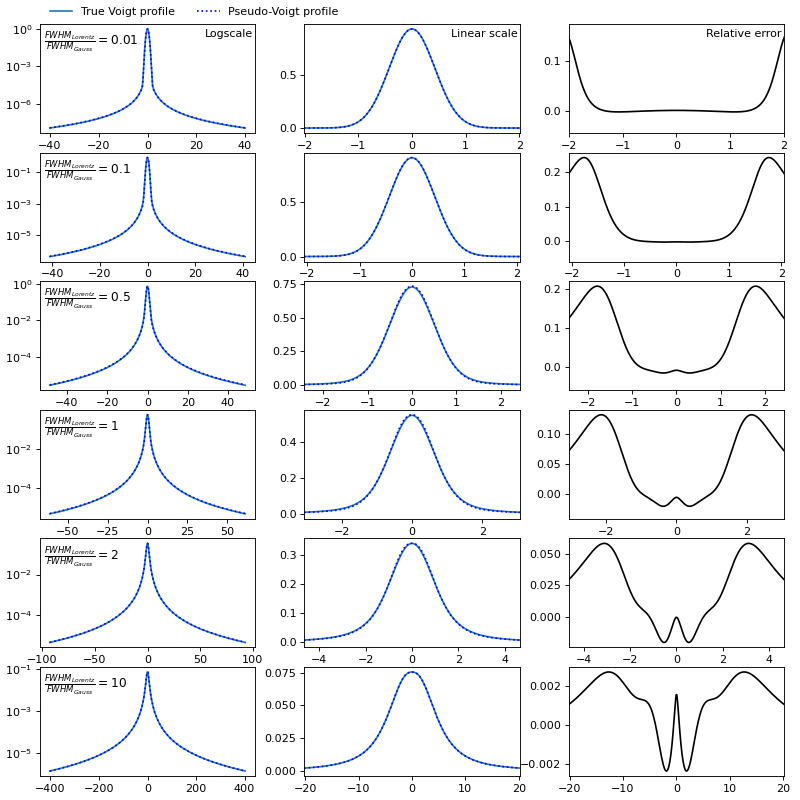
Calculating such a convolution for each spectral interval at each spatial point, given that thousands of paths are being traced, would take too much time. Therefore, I propose to replace this convolution with a weighted sum (so-called pseudo-Voigt):
$$V(\lambda-\lambda_0, \Delta\lambda_{1/2}^{(G)}, \Delta\lambda_{1/2}^{(L)})=\eta L(\lambda-\lambda_0, \Delta\lambda_{1/2}^{(V)}) + (1-\eta)G(\lambda-\lambda_0, \Delta\lambda_{1/2}^{(V)}),$$
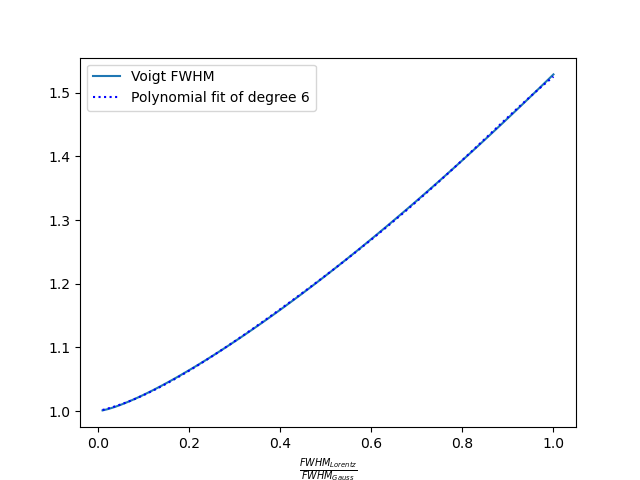
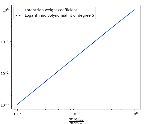
with $$\Delta\lambda_{1/2}^{(V)}\equiv F(\Delta\lambda_{1/2}^{(G)}, \Delta\lambda_{1/2}^{(L)}),$$ $$\eta\equiv f(\Delta\lambda_{1/2}^{(G)}, \Delta\lambda_{1/2}^{(L)}).$$
Both function, F and f can be obtained by fitting the true Voigt profile. The F function can be fitted with 6th degree polynomials of $$x=\frac{\Delta\lambda_{1/2}^{(L)}}{\Delta\lambda_{1/2}^{(G)}} \textrm{ for } \frac{\Delta\lambda_{1/2}^{(L)}}{\Delta\lambda_{1/2}^{(G)}} \le 1$$ $$\textrm{ and of } x=\frac{\Delta\lambda_{1/2}^{(G)}}{\Delta\lambda_{1/2}^{(L)}}\textrm{ for } \frac{\Delta\lambda_{1/2}^{(G)}}{\Delta\lambda_{1/2}^{(L)}} \le 1:$$

The f function can be fitted with 5th degree logarithmic polynomial of $$\frac{\Delta\lambda_{1/2}^{(L)}}{\Delta\lambda_{1/2}^{(V)}}$$ in the range from 0.01 to 0.999:
The maximum relative error of the pseudo-Voigt approximation can reach 25%, but all the main characteristics of the spectrum: maximum intensity, FWHM, line wings are approximated well.
Here is the script that does the above fitting:
pseudo_voigt_fit.py
import numpy as np
from scipy.special import wofz
from scipy.optimize import minimize, brentq, minimize_scalar
from matplotlib import pyplot as plt


def gaussian(x, sigma):
    return np.exp(-0.5 * x**2 / sigma**2) / (sigma * np.sqrt(2. * np.pi))


def lorentzian(x, lambda_1_2):
    return (0.5 / np.pi) * lambda_1_2 / (x**2 + (0.5 * lambda_1_2)**2)


def lorentzian25(x, lambda_1_2):
    """
    Modified Lorentzian from B. Lomanowski, et al. Nuclear Fusion 55.12 (2015)
    123028, https://doi.org/10.1088/0029-5515/55/12/123028
    """
    return (lambda_1_2**1.5 / 7.47443) / (np.abs(x)**2.5 + (0.5 * lambda_1_2)**2.5)


def voigt(x, sigma, lambda_1_2):
    """
    Exact computation of Voigt profile (gauss * lorentzian) using the Fadeeva function.
    Useful to test the convolution integration.

    :param x: Function argument.
    :param sigma: Gausian sigma.
    :param lambda_1_2: Lorentzian FWHM.
    """

    z = (x + 1j * 0.5 * lambda_1_2) / (sigma * np.sqrt(2))

    return np.real(wofz(z)) / (sigma * np.sqrt(2 * np.pi))


def voigt_convolution(x, fwhm_gauss, fwhm_lorentz, mg=512, ml=64, modified_lorentzian=True):
    """
    Computes Voigt profile as a convolution of Gaussian and Lorentzian profiles.

    :param x: Function argument.
    :param fwhm_gauss: Gausian FWHM.
    :param fwhm_lorentz: Lorentzian FWHM.
    :param mg: Number of grid points per Gausian FWHM. Default: 512.
    :param ml: Number of grid points per Lorentzian FWHM. Default: 64.
    :param modified_lorentzian: Use modified Lorentzian function. Default: True.
    """

    x = np.asarray(x)
    if x.ndim == 0:
        x = x[None]
    res = np.zeros(len(x))
    m = 8 * int(max(ml * fwhm_gauss / fwhm_lorentz, mg))
    x1, dx1 = np.linspace(- 4 * fwhm_gauss, 4 * fwhm_gauss, m, retstep=True)
    sigma = fwhm_gauss / (2 * np.sqrt(2 * np.log(2)))
    f1 = gaussian(x1, sigma)
    for ix, x0 in enumerate(x):
        f2 = lorentzian25(x1 - x0, fwhm_lorentz) if modified_lorentzian else lorentzian(x1 - x0, fwhm_lorentz)
        res[ix] = (f1 @ f2) * dx1

    return res


def pseudo_voigt(x, fwhm_gauss, fwhm_lorentz, voigt_fwhm_func, weight_func, modified_lorentzian=True):
    """
    Computes pseudo-Voigt profile as a weighted sum of Gaussian and lorentzian profiles.
    F_voigt(x) = weight * F_lorentz + (1. - weight) * F_gauss

    :param x: Function argument.
    :param fwhm_gauss: Gausian FWHM.
    :param fwhm_lorentz: Lorentzian FWHM.
    :param voigt_fwhm_func: A function of fwhm_gauss and fwhm_lorentz that returns
                            approximated Voigt FWHM, fwhm_voigt.
    :param weight_func: A function of fwhm_lorentz/fwhm_voigt that returns
                        a weight of Lorentzian profile.
    :param modified_lorentzian: Use modified Lorentzian function. Default: True.
    """

    fwhm = voigt_fwhm_func(fwhm_gauss, fwhm_lorentz)
    weight = weight_func(fwhm_lorentz / fwhm)

    sigma_v = 0.5 * fwhm / np.sqrt(2 * np.log(2))
    lorentz = lorentzian25(x, fwhm) if modified_lorentzian else lorentzian(x, fwhm)
    gs = gaussian(x, sigma_v)

    return weight * lorentz + (1 - weight) * gs


def voigt_find_fwhm(fwhm_gauss, fwhm_lorentz):
    """
    Finds Voigt FWHM.

    :param fwhm_gauss: Gausian FWHM.
    :param fwhm_lorentz: Lorentzian FWHM.
    """
    fvmax = voigt_convolution(0, fwhm_gauss, fwhm_lorentz)[0]

    def root_func(x):
        return voigt_convolution(x, fwhm_gauss, fwhm_lorentz)[0] - 0.5 * fvmax

    return 2. * brentq(root_func, 0, fwhm_gauss + fwhm_lorentz, maxiter=1000)


def fwhm_polyfit(x, y, deg):
    """
    Constrained polynomial fit: a0 = 1, a1 >= 0.
    """

    def min_func(w):
        fit = 1.
        for i, w1 in enumerate(w):
            fit += w1 * x**(i + 1)

        return ((1. - fit / y)**2).sum()

    constraints = [{'type': 'ineq', 'fun': lambda w: w[0]}]

    return np.append(minimize(min_func, np.zeros(deg), constraints=constraints).x[::-1], [1.])


def pseudo_voigt_fwhm_fit(deg_gauss=6, deg_lorentz=6, n=1000):
    """
    Fits Voigt FWHM with two polynoms of given degrees.

    For FWHM_{G} <= FWHM_{L}:
        FWHM_{V} = 1. + Sum_{i=1}^{N_{G}} a_i * (FWHM_{G}/FWHM_{L})^i

    For FWHM_{G} > FWHM_{L}:
        FWHM_{V} = 1. + Sum_{i=1}^{N_{L}} b_i * (FWHM_{L}/FWHM_{G})^i

    :param deg_gauss: N_{G}
    :param deg_lorentz: N_{L}
    :param n: FWHM_{G}/FWHM_{L} and FWHM_{L}/FWHM_{G} grid sizes.

    :returns: a_i, b_i
    """

    fwhm_gauss = np.geomspace(0.01, 1, n)
    fwhm_voigt = np.zeros(n)

    for i, g in enumerate(fwhm_gauss):
        fwhm_voigt[i] = voigt_find_fwhm(g, 1.)

    poly_gauss = fwhm_polyfit(fwhm_gauss, fwhm_voigt, deg_gauss)

    fwhm_lorentz = np.geomspace(0.01, 1, n)
    fwhm_voigt = np.zeros(n)

    for i, l in enumerate(fwhm_lorentz):
        fwhm_voigt[i] = voigt_find_fwhm(1., l)

    poly_lorentz = fwhm_polyfit(fwhm_lorentz, fwhm_voigt, deg_lorentz)

    return poly_gauss, poly_lorentz


def pseudo_voigt_weight_fit(fwhm_gauss, fwhm_lorentz, voigt_fwhm_func, n, relative=True):
    """
    Fits the Lorentzian weight in the pseudo-Voigt profile.

    :param fwhm_gauss: Gausian FWHM.
    :param fwhm_lorentz: Lorentzian FWHM.
    :param voigt_fwhm_func: A function of fwhm_gauss and fwhm_lorentz that returns
                            approximated Voigt FWHM.
    :param n: The argument grid size for fitting the pseudo-Voigt profile.
    :param relative: Relative (shape) or absolute (value) fit. Default: True (relative).
    """

    fwhm_voigt = voigt_fwhm_func(fwhm_gauss, fwhm_lorentz)

    if relative:
        x = np.geomspace(0.01 * fwhm_voigt, 50 * fwhm_voigt, n)
    else:
        x = np.linspace(0, 50 * fwhm_voigt, n)
    fv = voigt_convolution(x, fwhm_gauss, fwhm_lorentz)

    fl = lorentzian25(x, fwhm_voigt)
    fg = gaussian(x, 0.5 * fwhm_voigt / np.sqrt(2 * np.log(2)))

    def fit_func(x):
        return np.abs(fv - x * fl - (1. - x) * fg).sum()

    def rel_fit_func(x):
        return ((1. - (x * fl + (1. - x) * fg) / fv)**2).sum()

    f = rel_fit_func if relative else fit_func

    result = minimize_scalar(f, bounds=(0, 1), method='Bounded')

    return result.x


n = 8192
nw = 256

poly_gauss, poly_lorentz = pseudo_voigt_fwhm_fit(deg_gauss=6, deg_lorentz=6, n=1000)

poly_gauss_func = np.poly1d(poly_gauss)
poly_lorentz_func = np.poly1d(poly_lorentz)


def voigt_fwhm_func(fwhm_gauss, fwhm_lorentz):
    if fwhm_gauss > fwhm_lorentz:
        return fwhm_gauss * poly_lorentz_func(fwhm_lorentz / fwhm_gauss)

    return fwhm_lorentz * poly_gauss_func(fwhm_gauss / fwhm_lorentz)


fwhm_lorentz = np.geomspace(0.01, 100, nw)
weight = np.zeros(nw)
fwhm_ratio = np.zeros(nw)
for i in range(nw):
    fwhm_ratio[i] = fwhm_lorentz[i] / voigt_fwhm_func(1., fwhm_lorentz[i])
    print('Step {} out of {}. Fitting lorentzian weight for FWHM_lorentz/FWHM_Voigt = {}.'.format(i + 1, nw, fwhm_ratio[i]))
    weight[i] = pseudo_voigt_weight_fit(1., fwhm_lorentz[i], voigt_fwhm_func, n, relative=True)


deg = 5
poly_weight = np.polyfit(np.log(fwhm_ratio), np.log(weight), deg)


def weight_func(fwhm_ratio):
    return np.exp(np.poly1d(poly_weight)(np.log(fwhm_ratio)))


fwhm_gauss = np.linspace(0.01, 1., 100)
fwhm_voigt = np.array([voigt_find_fwhm(fg, 1.) for fg in fwhm_gauss])
fig = plt.figure()
ax = fig.add_subplot(111)
ax.plot(fwhm_gauss, fwhm_voigt, ls='-', c='tab:blue', label='Voigt FWHM')
ax.plot(fwhm_gauss, poly_gauss_func(fwhm_gauss), ls=':', c='b', label='Polynomial fit of degree {}'.format(6))
ax.set_xlabel(r'$\frac{FWHM_{Gauss}}{FWHM_{Lorentz}}$')
ax.legend(loc=0)

fwhm_lorentz = np.linspace(0.01, 1., 100)
fwhm_voigt = np.array([voigt_find_fwhm(1., fl) for fl in fwhm_lorentz])
fig = plt.figure()
ax = fig.add_subplot(111)
ax.plot(fwhm_lorentz, fwhm_voigt, ls='-', c='tab:blue', label='Voigt FWHM')
ax.plot(fwhm_lorentz, poly_lorentz_func(fwhm_lorentz), ls=':', c='b', label='Polynomial fit of degree {}'.format(6))
ax.set_xlabel(r'$\frac{FWHM_{Lorentz}}{FWHM_{Gauss}}$')
ax.legend(loc=0)

fig = plt.figure()
ax = fig.add_subplot(111)
ax.plot(fwhm_ratio, weight, ls='-', c='tab:blue', label='Lorentzian weight coefficient')
ax.plot(fwhm_ratio, weight_func(fwhm_ratio), ls=':', c='b', label='Logarithmic polynomial fit of degree {}'.format(deg))
ax.set_xlabel(r'$\frac{FWHM_{Lorentz}}{FWHM_{Voigt}}$')
ax.set_yscale('log')
ax.set_xscale('log')
ax.legend(loc=0)

fwhm_lorentz = [0.01, 0.1, 0.5, 1., 2., 10.]

fig = plt.figure(figsize=(10., 10.), dpi=80)

for i, fwhm_l in enumerate(fwhm_lorentz):
    fwhm_v = voigt_fwhm_func(1., fwhm_l)
    x = np.linspace(-40 * fwhm_v, 40 * fwhm_v, n)
    f_voigt = voigt_convolution(x, 1., fwhm_l)
    f_pseudo = pseudo_voigt(x, 1., fwhm_l, voigt_fwhm_func, weight_func)

    ax1 = fig.add_subplot(len(fwhm_lorentz), 3, 3 * i + 1)
    ax1.plot(x, f_voigt, ls='-', c='tab:blue', label='True Voigt profile')
    ax1.plot(x, f_pseudo, ls=':', c='b', label='Pseudo-Voigt profile')
    ax1.set_yscale('log')
    ax1.text(0.02, 0.95, r'$\frac{FWHM_{Lorentz}}{FWHM_{Gauss}} = $' + '{:g}'.format(fwhm_l), va='top', transform=ax1.transAxes, fontsize=11)

    ax2 = fig.add_subplot(len(fwhm_lorentz), 3, 3 * i + 2)
    ax2.plot(x, f_voigt, ls='-', c='tab:blue', label='True Voigt profile')
    ax2.plot(x, f_pseudo, ls=':', c='b', label='Pseudo-Voigt profile')
    ax2.set_xlim(-2 * fwhm_v, 2 * fwhm_v)

    ax3 = fig.add_subplot(len(fwhm_lorentz), 3, 3 * i + 3)
    ax3.plot(x, 1. - f_pseudo / f_voigt, ls='-', c='k', label='Residual')
    ax3.set_xlim(-2 * fwhm_v, 2 * fwhm_v)

    if i == 0:
        ax1.text(0.99, 0.95, 'Logscale', ha='right', va='top', transform=ax1.transAxes)
        ax2.text(0.99, 0.95, 'Linear scale', ha='right', va='top', transform=ax2.transAxes)
        ax3.text(0.99, 0.95, 'Relative error', ha='right', va='top', transform=ax3.transAxes)
        ax1.legend(loc=2, ncol=2, frameon=False, bbox_to_anchor=(0., 1.25))

fig.subplots_adjust(left=0.05, bottom=0.03, right=0.98, top=0.97, wspace=0.23, hspace=0.18)

plt.show()
As for the Zeeman effect, I think for now we can do the same as in Lomanowski B.A. et al, namely model Stark and Zeeman effects separately (each Zeeman component is a Stark-Doppler line). Later we can try to interpolate tabular data from J. Rosato, Y. Marandet, R. Stamm, Journal of Quantitative Spectroscopy & Radiative Transfer 187 (2017) 333, where both effects are taken into account simultaneously on quantum level.