Visualizing Decision Boundaries

[deepakgowtham]

Hi Aurelien,

Thanks a lot for your book, it helps me a lot to understand the basic concepts in a practical way. Can you please help me to understand the below code in general visualizing Decision Boundaries.

def plot_predictions(clf, axes):
    x0s = np.linspace(axes[0], axes[1], 100)
    x1s = np.linspace(axes[2], axes[3], 100)
    x0, x1 = np.meshgrid(x0s, x1s)
    X = np.c_[x0.ravel(), x1.ravel()]
    y_pred = clf.predict(X).reshape(x0.shape)
    y_decision = clf.decision_function(X).reshape(x0.shape)
    plt.contourf(x0, x1, y_pred, cmap=plt.cm.brg, alpha=0.2)
    plt.contourf(x0, x1, y_decision, cmap=plt.cm.brg, alpha=0.1)

plot_predictions(polynomial_svm_clf, [-1.5, 2.5, -1, 1.5])
plot_dataset(X, y, [-1.5, 2.5, -1, 1.5])

save_fig("moons_polynomial_svc_plot")
plt.show()

I understand that we create features using linspace to use them for getting predictions. But I am unable to understand how predictions in contourf visualizes decision boundary.

Also, regarding the part 2 of the book what steps should we follow to use with latest version of TensorFlow.

Thanks a lot in advance.

Regards Deepak.

[ageron]

Hi @deepakgowtham ,

Thanks for your questions, and I'm glad you're finding my book useful! 👍

First let's look at a simple example (try running it in a Jupyter notebook):

%matplotlib inline # only if you rum this in a Jupyter notebook
import matplotlib.pyplot as plt
import numpy as np

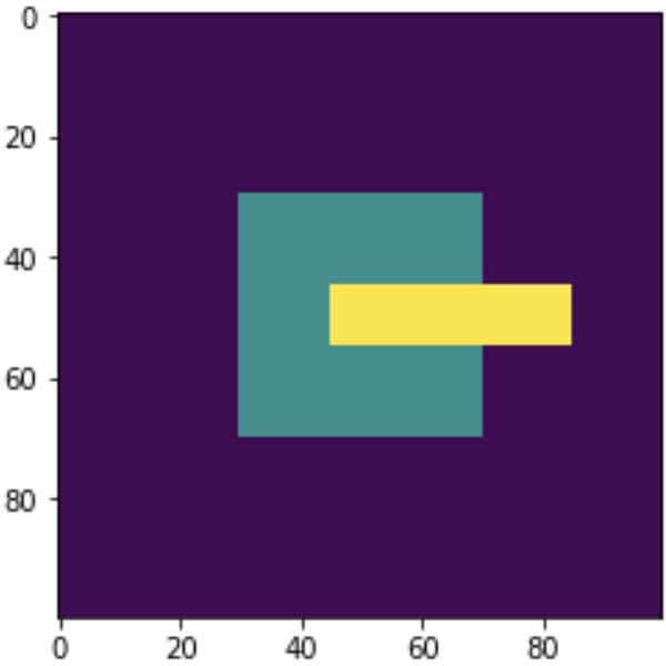
data = np.zeros([100, 100])
data[30:70, 30:70] = 1
data[45:55, 45:85] = 2
plt.imshow(data)
plt.show()

This creates a simple 2D NumPy array with values 0, 1, and 2, and displays it at an image:

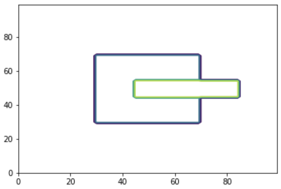
Now if I call plt.contour() instead of plt.imshow(), this is what I get:

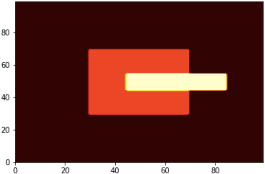
Then if I call plt.contourf() instead of plt.contour(), I get:

The aspect ratio is slightly different than using plt.imshow(), but it's basically the same image. Currently the value 0 maps to purple, the value 1 maps to blue-green, and value 2 maps to yellow. You can change the color map by setting the cmap argument. For example, if you set cmap="hot", you get this image:

Now we want to plot a diagram where each axis represents a different input feature, and the color represents the prediction. For this we start by calling np.linspace() to create an array of 100 different values between axes[0] and axes[1] for the first input features:

    x0s = np.linspace(axes[0], axes[1], 100)

Then we do the same for the second feature:

    x1s = np.linspace(axes[2], axes[3], 100)

Then we use np.meshgrid() to combine x1s and x2s, getting all the possible pairs of features from these arrays:

    x0, x1 = np.meshgrid(x0s, x1s)

A simple example might help understand what np.meshgrid() does:

>>> np.meshgrid([1,2,3], [4,5,6,7])
[array([[1, 2, 3],
        [1, 2, 3],
        [1, 2, 3],
        [1, 2, 3]]), array([[4, 4, 4],
        [5, 5, 5],
        [6, 6, 6],
        [7, 7, 7]])]

Then we flatten these two arrays into a 2D array containing all the possible pairs of features:

    X = np.c_[x0.ravel(), x1.ravel()]

If we were using features x1s=[1,2,3] and x2s=[4,5,6,7], then x0.ravel() would be [1,2,3,1,2,3,1,2,3,1,2,3], and x1.ravel() would be [4,4,4,5,5,5,6,6,6,7,7,7]. Therefore, X would be [[1,4], [2,4], [3,4], [1,5], [2,5], [3,5], [1,6], [2,6], [3,6], [1,7], [2,7], [3,7]]. It's basically a dataset containing all the possible combinations of features in the range we defined.

So now we can call the model's predict() method and reshape the result to obtain a 2D grid of the desired size:

    y_pred = clf.predict(X).reshape(x0.shape)

Now y_pred is a grid containing all the model's predictions for all the possible pairs of inputs. We can plot the result using plt.contourf():

    plt.contourf(x0, x1, y_pred, cmap=plt.cm.brg, alpha=0.2)

Hope this helps!

[ageron]

Note that the code overlays two contour plots: one for the "hard" predictions (positive class or negative class), and another for the prediction scores (returned by the model's decision_function() method). This makes it possible to see both in one diagram:

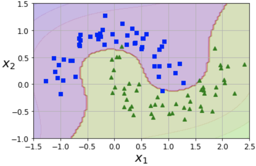
In order to see both, we need the contour plots to be slightly transparent. This is why we set alpha (that's the opacity level: 0=transparent, 1=opaque, 0.2=mostly transparent).

[deepakgowtham]

Thanks a lot for your reply Aurelien.

so in, plt.contourf(x0, x1, y_pred, cmap=plt.cm.brg, alpha=0.2) x0, x1 form the indices and y_pred provides the height, which in turn visualizes the decision boundary.

whereas in plt.contourf(data) we didnt provide the indices so the dimension of data was used as index.

Please correct me if I am wrong.

Also, Please let me know about the TensorFlow 2 Compatibility for part 2 of the book. How should I use the part 2 codes if using with latest version of TensorFlow.

Regards Deepak

[ageron]

Hi @deepakgowtham ,

Yes, you got it exactly right about the contourf() arguments.

Regarding TF 2 compatibility, if you want to run TF 1 code, the simplest option is just to install TF 1.15. You don't have to rush to TF 2.0. Check out this page for more details.

If you really want to run TF 1 code although you installed TF 2.0 or higher, then you need to run:

import tensorflow.compat.v1 as tf
tf.disable_v2_behavior()

Then make sure you replace tensorflow with tensorflow.compat.v1 in every import statement, for example, instead of:

from tensorflow.train import AdamOptimizer

You should write:

from tensorflow.compat.v1.train import AdamOptimizer

Unfortunately, if your TF 1 code uses tf.contrib, it won't work out of the box. You will need to upgrade the code that uses tf.contrib to use the equivalent TF 2 code, whenever possible (for example, the tf.contrib.eager.Variable class was moved to tf.Variable in TF 2, so you must run from tensorflow import Variable).

Other parts of tf.contrib were moved to the TensorFlow Addons project , such as the tf.contrib.image.rotate() function. You could install this project using pip install tensorflow-addons then import tensorflow_addons as tfa and use tfa.image.rotate().

Unfortunately, other parts of tf.contrib were just dropped, so you'll have to reimplement your code in some other way or copy the desired tf.contrib source code to your project.

Or... just downgrade to TF 1.15, it's probably much simpler.

Conversely, if you want to run TF 2 code in TF 1.14 or TF 1.15, it's possible:

import tensorflow.compat.v2 as tf
tf.enable_v2_behavior()

And replace tensorflow with tensorflow.compat.v2 in every import statement, for example instead of:

from tensorflow import keras

you must write:

from tensorflow.compat.v2 import keras

Hope this helps.

[deepakgowtham]

Thanks a lot @ageron. Your awesome replies motivates me study further more. Much oblieged.

Regards Deepak