Improve radar documentation/examples

[dopplershift]

• Since we now have azimuth_range_to_lat_lon, we should use that in the examples and actually plot the data on a map
• Tweak the docs to note that max_range is in km.

[dopplershift]

Also, looks like we have a bad 0-360 crossing in the level 2 example image that should be fixed:

[sgdecker]

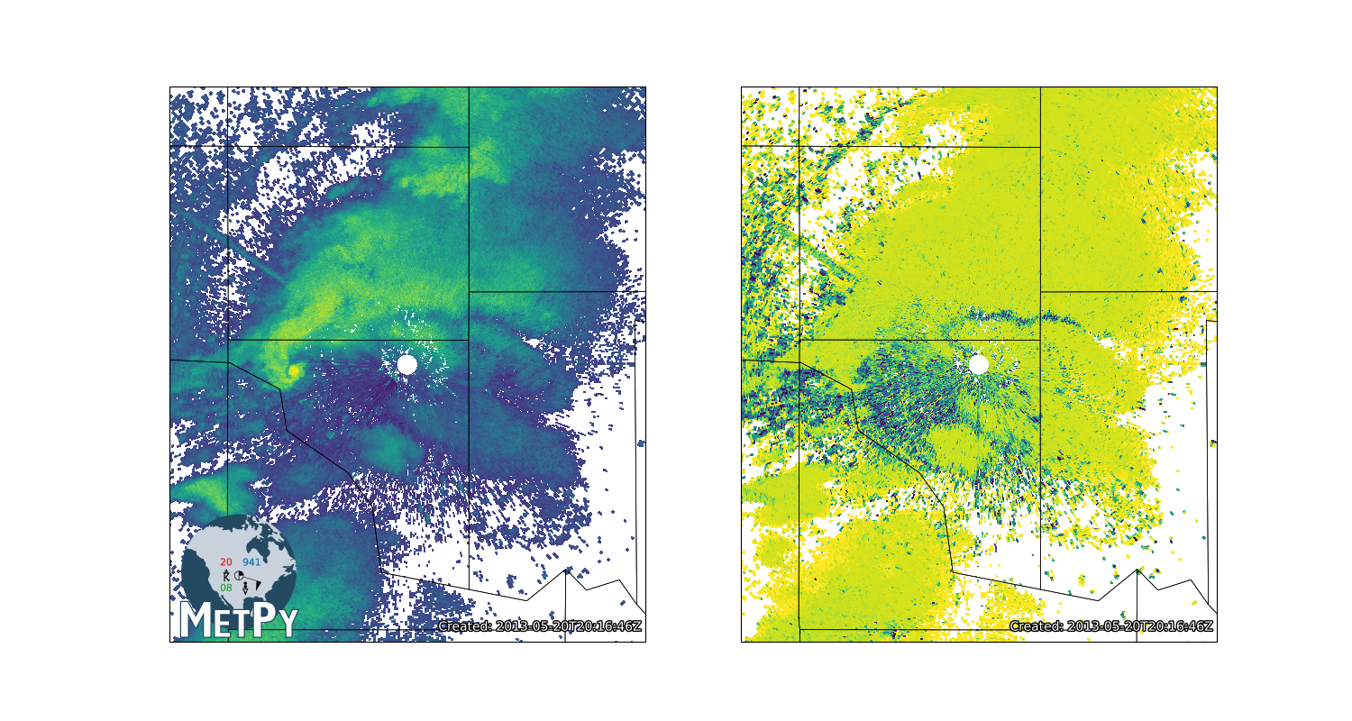
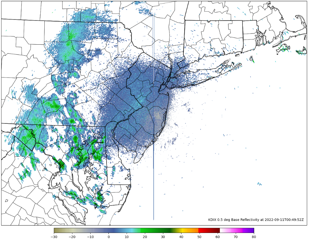
I have code (I think based on a MetPy example and another I found at some point) that does plot a radar image on a map, but it doesn't use azimuth_range_to_lat_lon, and it suffers from that north-south artifact. However, it may be a start:

import matplotlib.pyplot as plt
import numpy as np
from pyproj import Geod
import cartopy.crs as ccrs
import cartopy.feature as cfeature
from metpy.io import Level2File
from metpy.plots import colortables, add_timestamp, USCOUNTIES

rad_file = '/ldmdata/gempak/nexrad/craft/KDIX/KDIX_20220911_0049'
f = Level2File(rad_file)

rLAT = f.sweeps[0][0][1].lat
rLON = f.sweeps[0][0][1].lon

sweep = 0

az = np.array([ray[0].az_angle for ray in f.sweeps[sweep]])
diff = np.diff(az)
diff[diff > 180] -= 360.
diff[diff < -180] += 360.
avg_spacing = diff.mean()
az = (az[:-1] + az[1:]) / 2
az = np.concatenate(([az[0] - avg_spacing], az, [az[-1] + avg_spacing]))

ref_hdr = f.sweeps[sweep][0][4][b'REF'][0]
ref_range = (np.arange(ref_hdr.num_gates + 1) - 0.5) * ref_hdr.gate_width + ref_hdr.first_gate
ref = np.array([ray[4][b'REF'][1] for ray in f.sweeps[sweep]])

g = Geod(ellps='clrk66')
center_lat = np.ones([len(az), len(ref_range)])*rLAT
center_lon = np.ones([len(az), len(ref_range)])*rLON
az2D = np.ones_like(center_lat)*az[:, None]
rng2D = np.ones_like(center_lat)*np.transpose(ref_range[:, None])*1000
lon, lat, back = g.fwd(center_lon, center_lat, az2D, rng2D)

map_proj = ccrs.Gnomonic(central_latitude=rLAT, central_longitude=rLON)

fig, ax = plt.subplots(1, 1, figsize=(21.37, 14.37),
                       subplot_kw={'projection': map_proj})
data = np.ma.array(ref)
data[np.isnan(data)] = np.ma.masked

ax.add_feature(cfeature.STATES, linewidth=1)
ax.add_feature(USCOUNTIES, linewidth=.5)
cnorm, cmap = colortables.get_with_range(name='NWSStormClearReflectivity',
                                         start=-30, end=80)
mesh = ax.pcolormesh(lon, lat, data, cmap=cmap, norm=cnorm,
                     transform=ccrs.PlateCarree())
ax.set_extent((-78.6, -70.2, 37.5, 42.4))
fig.colorbar(mesh, orientation='horizontal', ticks=range(-30, 90, 10),
             shrink=.5, pad=.01, aspect=40)
add_timestamp(ax, f.dt, y=0.02, 
              pretext='KDIX 0.5 deg Base Reflectivity at ')
plt.show()

[dopplershift]

@sgdecker We updated the example to use azimuth_range_to_lat_lon in #2538. That's currently up on the dev docs, but no the released ones.

To deal with the north-south artifact from the 0-360 crossing, you need to deal with the fact that when doing az = (az[:-1] + az[1:]) / 2, the resulting angle can take the mean of ~0 and ~360, which -> 180. We really should be doing this in the data processing, when we improve the data model in #49.