Handle Constant Regions Consistently
Currently, stumpy.stump and stumpy.stumped can account for constant regions. So, when two subsequences are being compared and one subsequence is constant (and the second is not constant) then the pearson correlation is set to 0.5, which means that the z-normalized Euclidean distance is np.sqrt(np.abs(2 * m * (1 - 0.5))) or np.sqrt(m) (not sure if this is the best/correct choice see proof below). However, when both subsequences are constant then the pearson correlation is set to 1.0, which means that the distance is 0.0
However, this is unaccounted for in stumpy.mstump and stumpy.mstumped and stumpy.gpu_stump and stumpy.mass and some tests/naive.py implementatios. This may be something we should consider doing consistently everywhere.
changes to `_mass`
Replace the return statement with:
distance_profile = calculate_distance_profile(m, QT, μ_Q, σ_Q, M_T, Σ_T)
if σ_Q == 0.0:
    # Both subsequences are constant
    distance_profile[Σ_T == 0.0] = 0.0
else:
    # Only one subsequence is constant
    distance_profile[Σ_T == 0.0] = math.sqrt(m)

return distance_profile
This paper may offer some direction/insight as to how best to handle this.
@NimaSarajpoor @JaKasb When both subsequences are constant then we can say the z-norm distance is zero. Do you have any thoughts on how best to handle the situation when only one of the two subsequences are constant? What is reasonable in this case?
@seanlaw Very interesting. I have not read the paper yet. This is just what I think:
I think we should simply replace a constant subsequence with all zeros (after z-normalization).
So, let's say we have:
import numpy as np
s = np.full(m, a, dtype=np.float64)
Then, removing the offset (i.e. s_0 = s - s.mean()) becomes all 0. It does not matter what value of a we have.
Now, the question is: "How about standard deviation?" Because if we consider std=0, then s_0/0 is not defined. I THINK we can assume that std is very very small, and thus s_znorm = s_0 / std become 0. In fact, it does not matter what std we choose
as long as it is not zero, and I think it is okay! I think it is NOT meaningLESS.
So, let us say we have two other subsequences as follows:
# s2 --> has length m, mean 0, and it may look like a sine wave, with `std` of 1
# s3 --> has length m, mean 0, and it may look like a sine wave but with higher peak and lower valleys, with `std` of 2
# for instance: s3 = 2 * s2
it seems meaningful that d(s2, s3, normalize=True) is 0 (because they are similar). AND, it is also meaningful that their z-normalized distance to a constant subsequence s is basically the distance between their z-normalized version and an all-zero subsequence.
Please let me know if my explanation makes sense.
Another thing that just came to my mind and I thought it might be worth sharing:
The domain of z-normalized version of a non-constant subsequence with length m is R^{m} space excluding 0 (the origin). Replacing a constant subsequence with all-zero subsequence can make our domain cover the whole space.
@NimaSarajpoor So, to clarify the question, when both subsequences are constant then it is simple as the z-normalized distance between must be 0.0. However, what should the z-normalized euclidean distance be when only one subsequence is constant and the other subsequence is not constant? It is currently set to sqrt(m) and I can't recall where I got this from 😢 (see proof below)
Interestingly, I tried a "proof-by-simulation" and found that, for one constant subsequence (the second is random, non-constant), the z-normalized Euclidean distance is indeed sqrt(m)!!
import numpy as np
from numpy.linalg import norm
import math

m = 49
a = np.full(m, 10)
b = np.random.rand(m)

for i in range(6, 1000):
    a_std = math.pow(10, -i)
    D = norm(((a - a.mean())/a_std) - ((b - b.mean())/b.std()))
    print(a_std, D)
Click to expand and see printed results!
1e-06 7.000000000000001
1e-07 7.000000000000001
1e-08 7.000000000000001
1e-09 7.000000000000001
1e-10 7.000000000000001
1e-11 7.000000000000001
1e-12 7.000000000000001
1e-13 7.000000000000001
1e-14 7.000000000000001
1e-15 7.000000000000001
1e-16 7.000000000000001
1e-17 7.000000000000001
1e-18 7.000000000000001
1e-19 7.000000000000001
1e-20 7.000000000000001
1e-21 7.000000000000001
1e-22 7.000000000000001
1e-23 7.000000000000001
1e-24 7.000000000000001
1e-25 7.000000000000001
1e-26 7.000000000000001
1e-27 7.000000000000001
1e-28 7.000000000000001
1e-29 7.000000000000001
1e-30 7.000000000000001
1e-31 7.000000000000001
1e-32 7.000000000000001
1e-33 7.000000000000001
1e-34 7.000000000000001
1e-35 7.000000000000001
1e-36 7.000000000000001
1e-37 7.000000000000001
1e-38 7.000000000000001
1e-39 7.000000000000001
1e-40 7.000000000000001
1e-41 7.000000000000001
1e-42 7.000000000000001
1e-43 7.000000000000001
1e-44 7.000000000000001
1e-45 7.000000000000001
1e-46 7.000000000000001
1e-47 7.000000000000001
1e-48 7.000000000000001
1e-49 7.000000000000001
1e-50 7.000000000000001
1e-51 7.000000000000001
1e-52 7.000000000000001
1e-53 7.000000000000001
1e-54 7.000000000000001
1e-55 7.000000000000001
1e-56 7.000000000000001
1e-57 7.000000000000001
1e-58 7.000000000000001
1e-59 7.000000000000001
1e-60 7.000000000000001
1e-61 7.000000000000001
1e-62 7.000000000000001
1e-63 7.000000000000001
1e-64 7.000000000000001
1e-65 7.000000000000001
1e-66 7.000000000000001
1e-67 7.000000000000001
1e-68 7.000000000000001
1e-69 7.000000000000001
1e-70 7.000000000000001
1e-71 7.000000000000001
1e-72 7.000000000000001
1e-73 7.000000000000001
1e-74 7.000000000000001
1e-75 7.000000000000001
1e-76 7.000000000000001
1e-77 7.000000000000001
1e-78 7.000000000000001
1e-79 7.000000000000001
1e-80 7.000000000000001
1e-81 7.000000000000001
1e-82 7.000000000000001
1e-83 7.000000000000001
1e-84 7.000000000000001
1e-85 7.000000000000001
1e-86 7.000000000000001
1e-87 7.000000000000001
1e-88 7.000000000000001
1e-89 7.000000000000001
1e-90 7.000000000000001
1e-91 7.000000000000001
1e-92 7.000000000000001
1e-93 7.000000000000001
1e-94 7.000000000000001
1e-95 7.000000000000001
1e-96 7.000000000000001
1e-97 7.000000000000001
1e-98 7.000000000000001
1e-99 7.000000000000001
1e-100 7.000000000000001
1e-101 7.000000000000001
1e-102 7.000000000000001
1e-103 7.000000000000001
1e-104 7.000000000000001
1e-105 7.000000000000001
1e-106 7.000000000000001
1e-107 7.000000000000001
1e-108 7.000000000000001
1e-109 7.000000000000001
1e-110 7.000000000000001
1e-111 7.000000000000001
1e-112 7.000000000000001
1e-113 7.000000000000001
1e-114 7.000000000000001
1e-115 7.000000000000001
1e-116 7.000000000000001
1e-117 7.000000000000001
1e-118 7.000000000000001
1e-119 7.000000000000001
1e-120 7.000000000000001
1e-121 7.000000000000001
1e-122 7.000000000000001
1e-123 7.000000000000001
1e-124 7.000000000000001
1e-125 7.000000000000001
1e-126 7.000000000000001
1e-127 7.000000000000001
1e-128 7.000000000000001
1e-129 7.000000000000001
1e-130 7.000000000000001
1e-131 7.000000000000001
1e-132 7.000000000000001
1e-133 7.000000000000001
1e-134 7.000000000000001
1e-135 7.000000000000001
1e-136 7.000000000000001
1e-137 7.000000000000001
1e-138 7.000000000000001
1e-139 7.000000000000001
1e-140 7.000000000000001
1e-141 7.000000000000001
1e-142 7.000000000000001
1e-143 7.000000000000001
1e-144 7.000000000000001
1e-145 7.000000000000001
1e-146 7.000000000000001
1e-147 7.000000000000001
1e-148 7.000000000000001
1e-149 7.000000000000001
1e-150 7.000000000000001
1e-151 7.000000000000001
1e-152 7.000000000000001
1e-153 7.000000000000001
1e-154 7.000000000000001
1e-155 7.000000000000001
1e-156 7.000000000000001
1e-157 7.000000000000001
1e-158 7.000000000000001
1e-159 7.000000000000001
1e-160 7.000000000000001
1e-161 7.000000000000001
1e-162 7.000000000000001
1e-163 7.000000000000001
1e-164 7.000000000000001
1e-165 7.000000000000001
1e-166 7.000000000000001
1e-167 7.000000000000001
1e-168 7.000000000000001
1e-169 7.000000000000001
1e-170 7.000000000000001
1e-171 7.000000000000001
1e-172 7.000000000000001
1e-173 7.000000000000001
1e-174 7.000000000000001
1e-175 7.000000000000001
1e-176 7.000000000000001
1e-177 7.000000000000001
1e-178 7.000000000000001
1e-179 7.000000000000001
1e-180 7.000000000000001
1e-181 7.000000000000001
1e-182 7.000000000000001
1e-183 7.000000000000001
1e-184 7.000000000000001
1e-185 7.000000000000001
1e-186 7.000000000000001
1e-187 7.000000000000001
1e-188 7.000000000000001
1e-189 7.000000000000001
1e-190 7.000000000000001
1e-191 7.000000000000001
1e-192 7.000000000000001
1e-193 7.000000000000001
1e-194 7.000000000000001
1e-195 7.000000000000001
1e-196 7.000000000000001
1e-197 7.000000000000001
1e-198 7.000000000000001
1e-199 7.000000000000001
1e-200 7.000000000000001
1e-201 7.000000000000001
1e-202 7.000000000000001
1e-203 7.000000000000001
1e-204 7.000000000000001
1e-205 7.000000000000001
1e-206 7.000000000000001
1e-207 7.000000000000001
1e-208 7.000000000000001
1e-209 7.000000000000001
1e-210 7.000000000000001
1e-211 7.000000000000001
1e-212 7.000000000000001
1e-213 7.000000000000001
1e-214 7.000000000000001
1e-215 7.000000000000001
1e-216 7.000000000000001
1e-217 7.000000000000001
1e-218 7.000000000000001
1e-219 7.000000000000001
1e-220 7.000000000000001
1e-221 7.000000000000001
1e-222 7.000000000000001
1e-223 7.000000000000001
1e-224 7.000000000000001
1e-225 7.000000000000001
1e-226 7.000000000000001
1e-227 7.000000000000001
1e-228 7.000000000000001
1e-229 7.000000000000001
1e-230 7.000000000000001
1e-231 7.000000000000001
1e-232 7.000000000000001
1e-233 7.000000000000001
1e-234 7.000000000000001
1e-235 7.000000000000001
1e-236 7.000000000000001
1e-237 7.000000000000001
1e-238 7.000000000000001
1e-239 7.000000000000001
1e-240 7.000000000000001
1e-241 7.000000000000001
1e-242 7.000000000000001
1e-243 7.000000000000001
1e-244 7.000000000000001
1e-245 7.000000000000001
1e-246 7.000000000000001
1e-247 7.000000000000001
1e-248 7.000000000000001
1e-249 7.000000000000001
1e-250 7.000000000000001
1e-251 7.000000000000001
1e-252 7.000000000000001
1e-253 7.000000000000001
1e-254 7.000000000000001
1e-255 7.000000000000001
1e-256 7.000000000000001
1e-257 7.000000000000001
1e-258 7.000000000000001
1e-259 7.000000000000001
1e-260 7.000000000000001
1e-261 7.000000000000001
1e-262 7.000000000000001
1e-263 7.000000000000001
1e-264 7.000000000000001
1e-265 7.000000000000001
1e-266 7.000000000000001
1e-267 7.000000000000001
1e-268 7.000000000000001
1e-269 7.000000000000001
1e-270 7.000000000000001
1e-271 7.000000000000001
1e-272 7.000000000000001
1e-273 7.000000000000001
1e-274 7.000000000000001
1e-275 7.000000000000001
1e-276 7.000000000000001
1e-277 7.000000000000001
1e-278 7.000000000000001
1e-279 7.000000000000001
1e-280 7.000000000000001
1e-281 7.000000000000001
1e-282 7.000000000000001
1e-283 7.000000000000001
1e-284 7.000000000000001
1e-285 7.000000000000001
1e-286 7.000000000000001
1e-287 7.000000000000001
1e-288 7.000000000000001
1e-289 7.000000000000001
1e-290 7.000000000000001
1e-291 7.000000000000001
1e-292 7.000000000000001
1e-293 7.000000000000001
1e-294 7.000000000000001
1e-295 7.000000000000001
1e-296 7.000000000000001
1e-297 7.000000000000001
1e-298 7.000000000000001
1e-299 7.000000000000001
1e-300 7.000000000000001
1e-301 7.000000000000001
1e-302 7.000000000000001
1e-303 7.000000000000001
1e-304 7.000000000000001
1e-305 7.000000000000001
1e-306 7.000000000000001
1e-307 7.000000000000001
1e-308 7.000000000000001
1e-309 7.000000000000001
1e-310 7.000000000000001
1e-311 7.000000000000001
1e-312 7.000000000000001
1e-313 7.000000000000001
1e-314 7.000000000000001
1e-315 7.000000000000001
1e-316 7.000000000000001
1e-317 7.000000000000001
1e-318 7.000000000000001
1e-319 7.000000000000001
1e-320 7.000000000000001
1e-321 7.000000000000001
1e-322 7.000000000000001
1e-323 7.000000000000001
0.0 nan
0.0 nan
So, I am comfortable/confident that we can/should always set the z-normalized Euclidean distance to sqrt(m) when only one of the subsequences is constant
That is correct and it is aligned with the concept of replacing a constant subsequence with all 0. I will provide a link to its proof.
@seanlaw : I guess it´s correct if the other one is random. But as it is the case now in .mass() it is set to sqrt(m) independent of the other one which is not correct imho.
@seanlaw I tried to see if I can open the notebook in incognito mode (like when you want to open it on your end), and I couldn't. So, I submitted a PR so you can see the proof. Feel free to close/remove that PR after going through it and let me know if that makes sense.
@seanlaw And, one more thing: it would be nice if someone can read the paper and see if the authors investigate this matter further or not. I can read it if I get some free time in the future.
@seanlaw : I guess it´s correct if the other one is random. But as it is the case now in
.mass()it is set tosqrt(m)independent of the other one which is not correct imho.
Yes, this is not fixed in mass yet. This current issue, when resolved, would/should also require fixing mass too. Currently, only stump and stumped handle this correctly.
@seanlaw Update (might be of your interest)
I took a look at the paper. It seems it is about handling noise in time series data and how it affects the matrix profile distance. Apparently, noise has higher impact on flatter subsequences. So, if I understand correctly, their work is not about handling the constant subsequence S. It is about handling the subsequence S', where S' = S + noise, and S is constant.
See Section 4 Paragraph 1:
While the utility of the z-normalized Euclidean distance as a shape-comparator has been proven by the many Matrix Profile related publications [22, 24, 12], results become counter-intuitive for sequences that contain subsequences that are flat, with a small amount of noise.
The authors' observations sound interesting (see Fig. 4 and its caption), and this topic (i.e. handling noise) can have its own, separate issue if you think it's worth it. The core idea of paper is to (somehow?!) estimate \sigma_noise and then eliminate the impact of noise by modifying the z-normalized Euclidean Distances using formula provided in Algorithm1.
Thanks @NimaSarajpoor! I remember skimming the paper when it first came out and had the impression that it may be a "nice to have" (but not default) but not a "must have" because it isn't super obvious and adds some overhead. I only linked to the paper in case it could possibly help us deal with purely constant subsequences. I think the fix for this issue should be straightforward given the two cases.
@seanlaw I see. I am trying to figure out "HOW / WHY" this concept should be used when we are dealing with constant / almost constant subsequences. ~~So, for instance, we may add a noise to avoid divide-by-zero issue in z-normalizing constant subsequences, and then use the proposed method of paper to handle the noise!~~ As you noticed, it is not super obvious, and I think it needs some investigation on how it affects the results and if the final outcome is reasonable(?) or not.
A few notes
- I derived
eq(7)of paper, and it is correct. - The formula in Algorithm 1 has a typo. The correct one is provided in the section 3.2 of the author's previous work
- I think it is NOT CLEAR how they get from
eq(7)to the Formula proposed inAlgorithm1
Results
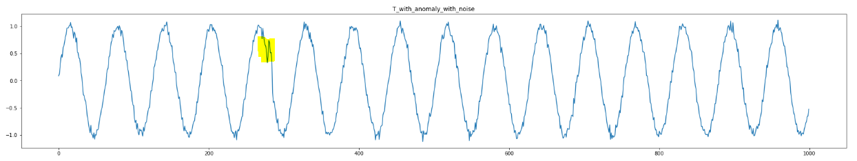
I also calculated the matrix profile of a noisy data that contains an anomaly, while considering Algorithm1 of paper (after fixing its typo).
# Generate sine wave
T = np.array(list(map(math.sin, np.linspace(0, 100, 1000))))


# Add anomaly at index 280, with length 5
anomaly_idx = 280
anomaly_width = 5

T_with_anomaly = T.copy()
T_with_anomaly[anomaly_idx : anomaly_idx + anomaly_width] += 0.5


# Add noise
n_T = len(T_with_anomaly)

seed = 0
np.random.seed(seed)
T_with_anomaly_with_noise =  T_with_anomaly.copy() + np.random.normal(0, 0.05, size=n_T)
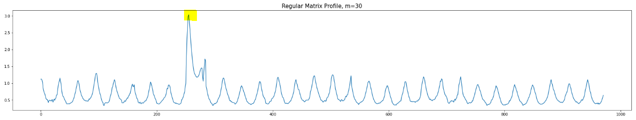
Now, let us plot the Regular Matrix Profile (i.e. no modification) and Modified Matrix Profile (i.e. considering noise elimination) below (m=8):

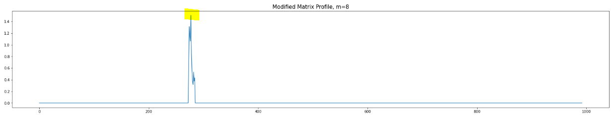
We can see the modified version can better detect anomaly for m=8.
Alternatively, as noted in the paper, we can just use Regular Matrix Profile but with bigger (longer) window size:
How to add it to stumpy.stump?
To use this in stumpy.stump, we can add parameter sigma_noise=0 and then, we can modify rho in O(1) time as follows:
Pearson_modified[i, j] = Pearson[i, j] + ( (1 + m) / m) * ( sigma_noise / (1e-06 + max(sigma_i, sigma_j)) ) ** 2
And, simply use Pearson_modified to update matrix profile and matrix profile indices.
An example on how we might handle constant subsequence cases
Let us take a look at the example below:
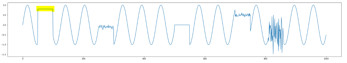
And, let us take a look at the distance profile of the highlighted subsequence shown above:
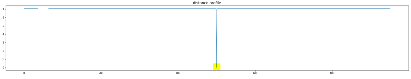
The match is the other constant subsequence in the data. But, we can see there are two other ALMOST constant subsequences. Now, let us take a look at the modified distance profile:

So, considering \sqrt(m) when one of the subsequences is constant might be too harsh(?!) and letting user play with sigma_noise might be useful!
@NimaSarajpoor Thank you for looking into this and for verifying that it does indeed work! To be clear, this current issue is focused on handling perfectly constant regions with zero noise but making sure that it is consistent across all z-normalized distance calculations as, right now, it is only handled in stumpy.stump and stumpy.stumped but missing in others. Let's track "constant regions with noise" in this other (original) issue.
Thanks for the clarification. I was actually trying to see if we can borrow an idea from the paper but I think I should better not go to that route. As you said before, the solutions discussed for the two cases for constant subsequences should suffice. (I was wondering if there is something more that you may have in mind)
I also found the results interesting but didn't know there was an issue about this before. Thanks for reopening that! I have some thoughts about handling noise and I will share them in that issue. Sorry for going off-road in this issue.
I also expiremented the with the noise compensation method: Many aspects in the realm of matrix profiles algorithms suffer from instability in edge cases:
How to choose sigma_n ?
Set sigma_n too small and the correction has no effect. Set sigma_n too large and the correction overshoots and results in negative euclidean distances. Even with reasonable sigma_n, the compensation needs safeguard measures to protect against negative distances. I derived a supremum for sigma_n, by assuming Pearson Correlation of -1 and solving for sigma_n in E[D²] = max_possible_distance²
_denom = np.maximum(sigma_i, sigma_j)**2
# https://www.wolframalpha.com/input?i=solve+%282*m+%2B+2%29+*%28x%5E2%29%2F%28d%29+%3D+4m+for+x+and+d%3E0+and+m%3E0
supremum_sigma_n = np.sqrt(2) * np.sqrt(_denom*m/(m+1))
sigma_n = np.clip(sigma_n, a_min=0, a_max=supremum_sigma_n)
E_d_squared_max = (2*m + 2)*(supremum_sigma_n**2)/_denom
assert np.allclose(E_d_squared_max, 4*m)
However, this upper limit on sigma_n is useless in practice, because the expected value of the pearson correlation is ca 0, as opposed to -1.
Assumptions
The method flatout assumes Gaussian Noise, however constant subsequences often stem from quantization errors. The probability density function of the quantization error is Uniform instead of Gaussian. https://www.allaboutcircuits.com/technical-articles/quantization-nois-amplitude-quantization-error-analog-to-digital-converters/
Comparison to Annotation Vector
The noise compensation method can be interpreted as a special case of the Annotaion Vector framework.
https://dl.acm.org/doi/pdf/10.1145/3097983.3097993
Corrected Distance = dist + (1-AV)*max_distance
compared to
corrected distance = sqrt(dist² - E[D²]
The negative of E[D²] is an Annotation Vector.
Because E[D²] can be reduced to: constant_factor * 1/np.std(subsequence) :
The benefit of the AV-framework is that the AV is normalized to 0..1, therefore the constant factor is less of a problem, therefore the choice of sigma_n is not as sensitive.
Comparison to CID
https://www.researchgate.net/publication/254861501_CID_An_efficient_complexity-invariant_distance_for_time_series As a reminder, the time series complexity measure is the "length" of a time-series if the time series were a rope. I assume that E[D] and Complexity are highly correlated: If the subsequence is flat the complexity is low and std() are low. If the subsequence is squiggly, then the complexity and std() are high. EDIT: A quick experiment shows only weak correlation ?!
Choice of Expected-Value as predictor
The Expected Value is a good predictor if both subsequences are noise and uncorrelated. In the case of a perfect motif match (euclidean distance = 0) the Expected Value is very off. Analyzing the histogramm of euclidean distances can be very misleading, because the motif-matches are strong outliers in the overall histogramm. The matrix-profile lies the outer edge of the fat tails of the distance histogramm. There are some papers that study the histogram of the distance-matrix and the matrix profiles, but that only works on some types of time series. Maybe a Baysian Interpretation could be helpful ? (Given sigma_x and sigma_y how likely is the observed euclidean distance ?)