Problem solving time-dependent PDE with Neumann BCs

[killah-t-cell]

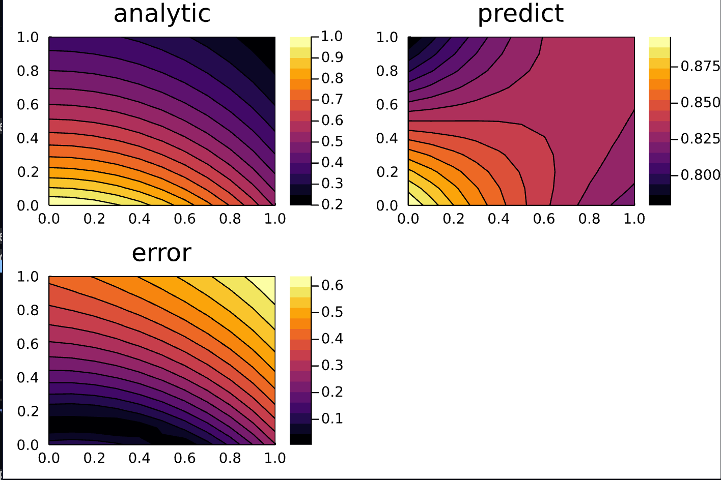
I just tried to solve a hyperbolic equation with Neumann BCs using adaptive derivative. Unfortunately, it performed badly. The version without the adaptive derivative performed the same. I tried several training strategies and in this case, QuasiRandomTraining worked the best.

My guess is this is related to adding time. It seems that once you add time, you need to add the analytical solution to the boundary conditions to prevent bad results. You do that here https://neuralpde.sciml.ai/stable/pinn/2D/. I did this here https://neuralpde.sciml.ai/stable/pinn/system/. So Neumann BCs wouldn't perform well with the current solver.

It seems that in order to handle time, we need to either use a moving time window approach or implement an LSTM (or both?).

Here is my code for reference

# Parameters, variables, and derivatives
@parameters t x
@variables u(..), Dxu(..), Dtu(..), O1(..), O2(..)
Dt = Differential(t) 
Dx = Differential(x) 
Dxx = Differential(x)^2 

# PDE and boundary conditions
eq  = Dtu(t, x) ~ Dx(Dxu(t, x))
bcs_ = [u(0, x) ~ cos(x),
       Dxu(t, 0) ~ 0,
       Dxu(t, 1) ~ 0]

ep = (cbrt(eps(eltype(Float64))))^2 / 6

der = [Dxu(t, x) ~ Dx(u(t, x)) + ep * O1(t, x),
       Dtu(t, x) ~  Dt(u(t, x)) + ep * O2(t, x)]

bcs = [bcs_;der]

# Space and time domains
domains = [t ∈ Interval(0.0, 1.0),
           x ∈ Interval(0.0, 1.0)]

# Neural network
chain = [[FastChain(FastDense(2, 12, Flux.tanh), FastDense(12, 12, Flux.tanh), FastDense(12, 1)) for _ in 1:3];
         [FastChain(FastDense(2, 4, Flux.tanh), FastDense(4, 1)) for _ in 1:2];]
         
quasirandom_strategy = NeuralPDE.QuasiRandomTraining(1000; # points
                                                     sampling_alg=LatinHypercubeSample())
initθ = map(c -> Float64.(c), DiffEqFlux.initial_params.(chain))

discretization = NeuralPDE.PhysicsInformedNN(chain, quasirandom_strategy;init_params=initθ)
pde_system = PDESystem(eq, bcs, domains, [t, x], [u,Dxu,Dtu,O1,O2])
prob = NeuralPDE.discretize(pde_system, discretization)
sym_prob = NeuralPDE.symbolic_discretize(pde_system, discretization)

pde_inner_loss_functions = prob.f.f.loss_function.pde_loss_function.pde_loss_functions.contents
bcs_inner_loss_functions = prob.f.f.loss_function.bcs_loss_function.bc_loss_functions.contents

cb_ = function (p, l)
    println("loss: ", l)
    println("pde_losses: ", map(l_ -> l_(p), pde_inner_loss_functions))
    println("bcs_losses: ", map(l_ -> l_(p), bcs_inner_loss_functions))
    return false
end

res = GalacticOptim.solve(prob, BFGS(); cb=cb, maxiters=100)
phi = discretization.phi[1]


# Analysis
ts, xs = [infimum(d.domain):dx:supremum(d.domain) for d in domains]
analytic_sol_func(x, t) = exp.(-t) * cos.(x)

# Plot
using Plots
using Printf

u_predict = reshape([first(phi([t,x], res.minimizer)) for t in ts for x in xs], (length(ts), length(xs)))
u_real = reshape([analytic_sol_func(t, x) for t in ts for x in xs], (length(ts), length(xs)))

diff_u = abs.(u_predict .- u_real)
p1 = plot(ts, xs, u_real, linetype=:contourf, title="analytic");
p2 = plot(ts, xs, u_predict, linetype=:contourf, title="predict");
p3 = plot(ts, xs, diff_u, linetype=:contourf, title="error");
plot(p1,p2,p3)

using NeuralPDE, Flux, ModelingToolkit, GalacticOptim, Optim, DiffEqFlux
using Plots
using Quadrature, Cuba, QuasiMonteCarlo
import ModelingToolkit: Interval, infimum, supremum

# Parameters, variables, and derivatives
@parameters t x
@variables u(..)
Dt = Differential(t) 
Dx = Differential(x) 
Dxx = Differential(x)^2 

# 1D PDE and boundary conditions
eq  = Dt(u(t, x)) ~ Dxx(u(t, x))
bcs = [u(0, x) ~ cos(x),
       Dx(u(t, 0)) ~ 0,
       Dx(u(t, 1)) ~ 0]

# Space and time domains
domains = [t ∈ Interval(0.0, 1.0),
           x ∈ Interval(0.0, 1.0)]

# Neural network
chain = FastChain(FastDense(2, 16, Flux.σ), FastDense(16, 16, Flux.σ), FastDense(16, 1))
initθ = map(c -> Float64.(c), DiffEqFlux.initial_params.(chain))

quasirandom_strategy = NeuralPDE.QuasiRandomTraining(100; sampling_alg=LatinHypercubeSample())
discretization = NeuralPDE.PhysicsInformedNN(chain, GridTraining(0.01);init_params=initθ)
pde_system = PDESystem(eq, bcs, domains, [t, x], [u])
prob = NeuralPDE.discretize(pde_system, discretization)
sym_prob = NeuralPDE.symbolic_discretize(pde_system, discretization)

pde_inner_loss_functions = prob.f.f.loss_function.pde_loss_function.pde_loss_functions.contents
bcs_inner_loss_functions = prob.f.f.loss_function.bcs_loss_function.bc_loss_functions.contents

cb_ = function (p, l)
    println("loss: ", l)
    println("pde_losses: ", map(l_ -> l_(p), pde_inner_loss_functions))
    println("bcs_losses: ", map(l_ -> l_(p), bcs_inner_loss_functions))
    return false
end

res = GalacticOptim.solve(prob, BFGS(); cb=cb, maxiters=1000)
phi = discretization.phi


# Analysis
ts, xs = [infimum(d.domain):0.1:supremum(d.domain) for d in domains]

analytic_sol_func(x, t) = exp.(-t) * cos.(x)

# Plot
using Plots
using Printf

u_predict = reshape([first(phi([t,x], res.minimizer)) for t in ts for x in xs], (length(ts), length(xs)))
u_real = reshape([analytic_sol_func(t, x) for t in ts for x in xs], (length(ts), length(xs)))

diff_u = abs.(u_predict .- u_real)
p1 = plot(ts, xs, u_real, linetype=:contourf, title="analytic");
p2 = plot(ts, xs, u_predict, linetype=:contourf, title="predict");
p3 = plot(ts, xs, diff_u, linetype=:contourf, title="error");
plot(p1,p2,p3)

[killah-t-cell]

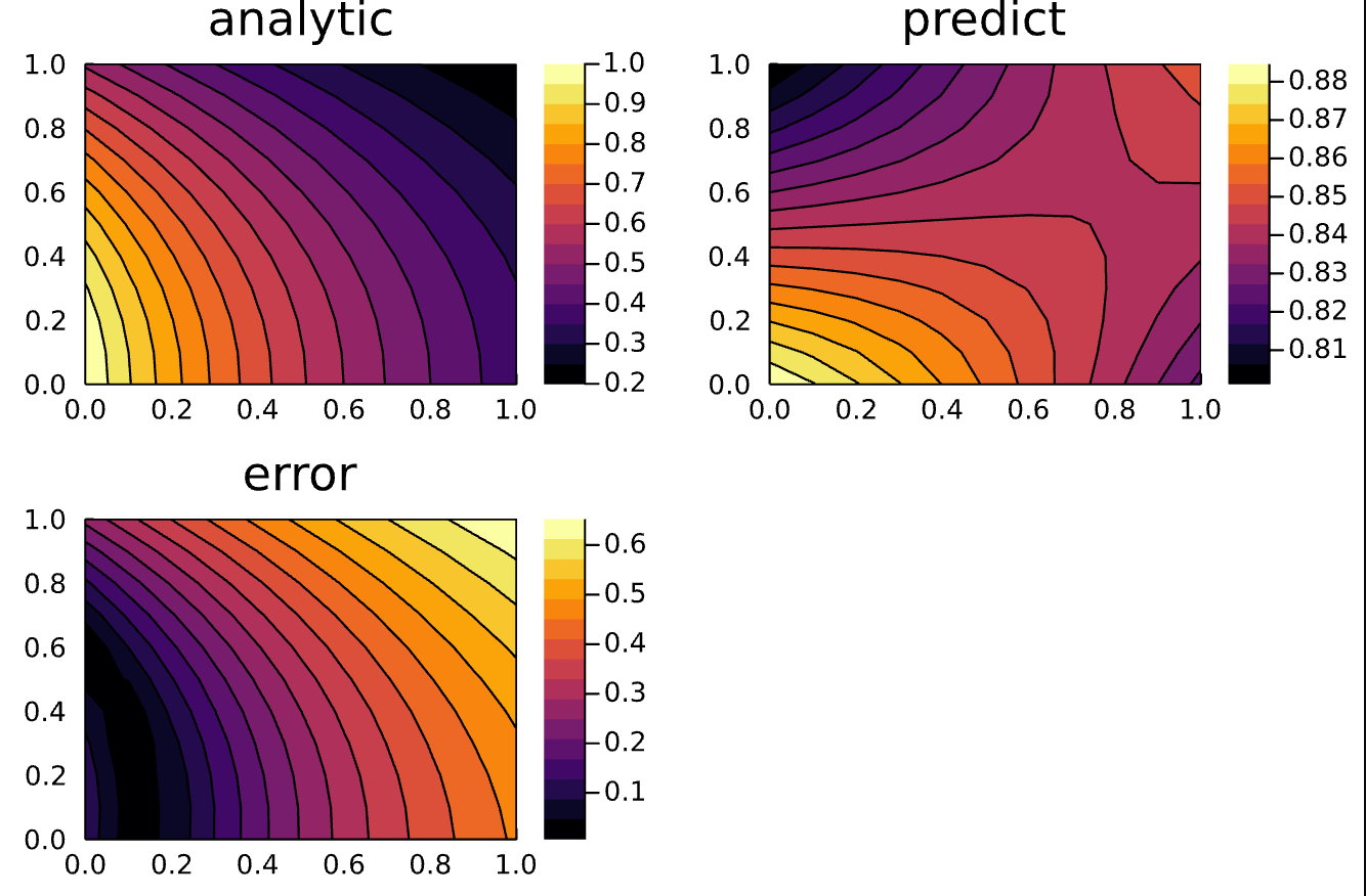
Just tried optimizing with ADAM + BFGS and that didn't work well either just fyi :)

[ChrisRackauckas]

It seems that in order to handle time, we need to either use a moving time window approach or implement an LSTM (or both?).

It does help. Did you try it out?

[killah-t-cell]

@ChrisRackauckas I'm not sure I know how to. How does one go about doing that?

[ChrisRackauckas]

There should be multiple tutorials which show it IIRC.

res = GalacticOptim.solve(prob, ADAM(); cb=cb, maxiters=300)
res = GalacticOptim.solve(remake(prob, p = res.minimizer), BFGS(); cb=cb, maxiters=1000)
phi = discretization.phi

[killah-t-cell]

@ChrisRackauckas I will look them up. I had tried something similar (it's what I mean by ADAM + BFGS) and it definitely got me closer but it still struggled to approximate.

Here is the updated code for reference:

using NeuralPDE, Flux, ModelingToolkit, GalacticOptim, Optim, DiffEqFlux
using Plots
using Quadrature, Cuba, QuasiMonteCarlo
import ModelingToolkit: Interval, infimum, supremum

# Parameters, variables, and derivatives
@parameters t x
@variables u(..)
Dt = Differential(t) 
Dx = Differential(x) 
Dxx = Differential(x)^2 

# 1D PDE and boundary conditions
eq  = Dt(u(t, x)) ~ Dxx(u(t, x))
bcs = [u(0, x) ~ cos(x),
       Dx(u(t, 0)) ~ 0,
       Dx(u(t, 1)) ~ 0]

# Space and time domains
domains = [t ∈ Interval(0.0, 1.0),
           x ∈ Interval(0.0, 1.0)]

# Neural network
chain = FastChain(FastDense(2, 16, Flux.σ), FastDense(16, 16, Flux.σ), FastDense(16, 1))
initθ = map(c -> Float64.(c), DiffEqFlux.initial_params.(chain))

quasirandom_strategy = NeuralPDE.QuasiRandomTraining(500; sampling_alg=LatinHypercubeSample())
discretization = NeuralPDE.PhysicsInformedNN(chain, quasirandom_strategy;init_params=initθ)
pde_system = PDESystem(eq, bcs, domains, [t, x], [u])
prob = NeuralPDE.discretize(pde_system, discretization)

pde_inner_loss_functions = prob.f.f.loss_function.pde_loss_function.pde_loss_functions.contents
bcs_inner_loss_functions = prob.f.f.loss_function.bcs_loss_function.bc_loss_functions.contents

cb_ = function (p, l)
    println("loss: ", l)
    println("pde_losses: ", map(l_ -> l_(p), pde_inner_loss_functions))
    println("bcs_losses: ", map(l_ -> l_(p), bcs_inner_loss_functions))
    return false
end

ts, xs = [infimum(d.domain):0.1:supremum(d.domain) for d in domains]

res = GalacticOptim.solve(prob, ADAM(); cb=cb, maxiters=300)
res = GalacticOptim.solve(remake(prob, p=res.minimizer), BFGS(); cb=cb, maxiters=1000)
phi = discretization.phi

# Analysis

analytic_sol_func(t, x) = exp.(-t) * cos.(x)

# Plot
u_predict = reshape([first(phi([t,x], res.minimizer)) for t in ts for x in xs], (length(ts), length(xs)))
u_real = reshape([analytic_sol_func(t, x) for t in ts for x in xs], (length(ts), length(xs)))

diff_u = abs.(u_predict .- u_real)
p1 = plot(ts, xs, u_real, linetype=:contourf, title="analytic");
p2 = plot(ts, xs, u_predict, linetype=:contourf, title="predict");
p3 = plot(ts, xs, diff_u, linetype=:contourf, title="error");
plot(p1, p2, p3)
savefig("bc_homogeneous")


@assert u_predict ≈ u_real atol = 10^-4

[KirillZubov]

it's typo in bound cond

bcs = [u(0, x) ~ cos(x),
       Dx(u(t, 0)) ~ 0,
       Dx(u(t, 1)) ~ exp(-t) * -sin(1)]
analytic_sol_func(t, x) = exp.(-t) * cos.(x)

[KirillZubov]

and here remake(prob, p=res.minimizer) correct remake(prob, u0=res.minimizer)

[KirillZubov]

# Parameters, variables, and derivatives
@parameters t x
@variables u(..)
Dt = Differential(t)
Dx = Differential(x)
Dxx = Differential(x)^2

# 1D PDE and boundary conditions
eq  = Dt(u(t, x)) ~ Dxx(u(t, x))
bcs = [u(0, x) ~ cos(x),
       Dx(u(t, 0)) ~ 0,
       Dx(u(t, 1)) ~ exp(-t) * -sin(1)]
analytic_sol_func(t, x) = exp.(-t) * cos.(x)
# Space and time domains
domains = [t ∈ Interval(0.0, 1.0),
           x ∈ Interval(0.0, 1.0)]

# Neural network
chain = FastChain(FastDense(2, 16, Flux.σ), FastDense(16, 16, Flux.σ), FastDense(16, 1))
initθ = map(c -> Float64.(c), DiffEqFlux.initial_params.(chain))

strategy = NeuralPDE.QuadratureTraining()
# strategy = NeuralPDE.GridTraining(0.1)
discretization = NeuralPDE.PhysicsInformedNN(chain, strategy;init_params=initθ)
pde_system = PDESystem(eq, bcs, domains, [t, x], [u])
prob = NeuralPDE.discretize(pde_system, discretization)

pde_inner_loss_functions = prob.f.f.loss_function.pde_loss_function.pde_loss_functions.contents
bcs_inner_loss_functions = prob.f.f.loss_function.bcs_loss_function.bc_loss_functions.contents

cb_ = function (p, l)
    println("loss: ", l)
    println("pde_losses: ", map(l_ -> l_(p), pde_inner_loss_functions))
    println("bcs_losses: ", map(l_ -> l_(p), bcs_inner_loss_functions))
    return false
end

ts, xs = [infimum(d.domain):0.1:supremum(d.domain) for d in domains]

res = GalacticOptim.solve(prob, BFGS(); cb=cb, maxiters=1000)
prob =remake(prob, u0=res.minimizer)
res = GalacticOptim.solve(prob, ADAM(0.01); cb=cb, maxiters=1000)
prob =remake(prob, u0=res.minimizer)
res = GalacticOptim.solve(prob, BFGS(); cb=cb, maxiters=1000)
phi = discretization.phi

analytic_sol_func(t, x) = exp.(-t) * cos.(x)

# Plot
u_predict = reshape([first(phi([t,x], res.minimizer)) for t in ts for x in xs], (length(ts), length(xs)))
u_real = reshape([analytic_sol_func(t, x) for t in ts for x in xs], (length(ts), length(xs)))

diff_u = abs.(u_predict .- u_real)
p1 = plot(ts, xs, u_real, linetype=:contourf, title="analytic");
p2 = plot(ts, xs, u_predict, linetype=:contourf, title="predict");
p3 = plot(ts, xs, diff_u, linetype=:contourf, title="error");
plot(p1, p2, p3)

@assert u_predict ≈ u_real atol = 10^-4

[KirillZubov]

and with adapt derevative. the coolest thing in adaptive der that we are not limited by the accuracy of the derivative algorithm

@parameters t x
@variables u(..), Dxu(..) O1(..)
Dt = Differential(t)
Dx = Differential(x)
Dxx = Differential(x)^2

# PDE and boundary conditions
eq  = Dt(u(t, x)) ~ Dx(Dxu(t, x))

bcs_ = [u(0, x) ~ cos(x),
       Dx(u(t, 0)) ~ 0,
       Dx(u(t, 1)) ~ exp(-t) * -sin(1)]

ep = (cbrt(eps(eltype(Float64))))^2 / 6

der = [Dxu(t, x) ~ Dx(u(t, x)) + ep * O1(t, x)]

bcs = [bcs_;der]

# Space and time domains
domains = [t ∈ Interval(0.0, 1.0),
           x ∈ Interval(0.0, 1.0)]

# Neural network
chain = [[FastChain(FastDense(2, 16, Flux.tanh), FastDense(16, 16, Flux.tanh), FastDense(16, 1)) for _ in 1:2];
         [FastChain(FastDense(2, 6, Flux.tanh), FastDense(6, 1)) for _ in 1:1];]

initθ = map(c -> Float64.(c), DiffEqFlux.initial_params.(chain))

strategy = NeuralPDE.GridTraining(0.05)
discretization = NeuralPDE.PhysicsInformedNN(chain, strategy;init_params=initθ)
pde_system = PDESystem(eq, bcs, domains, [t, x], [u,Dxu,O1])
prob = NeuralPDE.discretize(pde_system, discretization)
sym_prob = NeuralPDE.symbolic_discretize(pde_system, discretization)

pde_inner_loss_functions = prob.f.f.loss_function.pde_loss_function.pde_loss_functions.contents
bcs_inner_loss_functions = prob.f.f.loss_function.bcs_loss_function.bc_loss_functions.contents

cb_ = function (p, l)
    println("loss: ", l)
    println("pde_losses: ", map(l_ -> l_(p), pde_inner_loss_functions))
    println("bcs_losses: ", map(l_ -> l_(p), bcs_inner_loss_functions))
    return false
end


res = GalacticOptim.solve(prob, BFGS(); cb=cb_, maxiters=1000)
prob =remake(prob, u0=res.minimizer)
res = GalacticOptim.solve(prob, BFGS(); cb=cb_, maxiters=3000)

# discretization = NeuralPDE.PhysicsInformedNN(chain,NeuralPDE.QuasiRandomTraining(500; sampling_alg=LatinHypercubeSample()))
# prob =remake(prob, discretization=discretization)
# prob =remake(prob, u0=res.minimizer)
# res = GalacticOptim.solve(prob, ADAM(0.01); cb=cb, maxiters=1000)
# prob =remake(prob, u0=res.minimizer)
# res = GalacticOptim.solve(prob, BFGS();abstol=1e-15, cb=cb, maxiters=1000)
# ,reltol =10^-20
phi = discretization.phi[1]

# Analysis
ts, xs = [infimum(d.domain):dx:supremum(d.domain) for d in domains]
analytic_sol_func(t, x) = exp.(-t) * cos.(x)

# Plot
using Plots
using Printf

u_predict = reshape([first(phi([t,x], res.minimizer)) for t in ts for x in xs], (length(ts), length(xs)))
u_real = reshape([analytic_sol_func(t, x) for t in ts for x in xs], (length(ts), length(xs)))

diff_u = abs.(u_predict .- u_real)
p1 = plot(ts, xs, u_real, linetype=:contourf, title="analytic");
p2 = plot(ts, xs, u_predict, linetype=:contourf, title="predict");
p3 = plot(ts, xs, diff_u, linetype=:contourf, title="error");
plot(p1,p2,p3)

[killah-t-cell]

Ah of course. That was silly of me. Thanks for finding this.

[killah-t-cell]

Should I add this to the documentation? If so, where? @KirillZubov

[KirillZubov]

@killah-t-cell we going to update the doc so I will add the example together with the update.