MTK -- weird solution with step inputs

[B-LIE]

Frequently, MTK models exhibit weird/unphysical oscillatoric behavior when I use step inputs and default solvers:

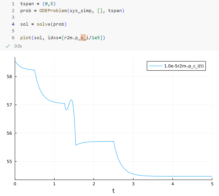
This plot uses input functions:

u_p_f(t) = t < 0.5 ? 220e5 : 0.95*220e5
u_p_m(t) = t < 1.5 ? 50e5 : 0.97*50e5
u_f_p(t) = t < 2.5 ? 60 : 0.95*60
u_χ_w(t) = 0.35

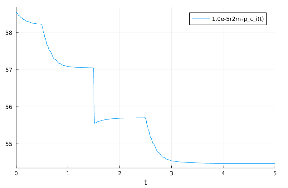
Observe that the oscillation starts prior to the temporal location of one of the step changes. It is as if a too infrequent sampling is used, in combination with the built-in interpolation of the solution.

I have tried to specify tstops at the location of the step changes, without any improvement. I have also tried to specify a high resolution saveat, without any improvement.

The displayed behavior shows up when I use the default solver. I have tried to specify other solvers. The solvers I typically end up with are the BDF solvers, e.g., QBDF. With this solver, I get a more realistic solution:

This solution is somewhat jagged; the solution gets better if I set reltol to 1e-4 or smaller.

• Question: what is the cause of this strange, oscillatory solution? Is there a way to fix it using the default solver?

If you need my code to figure out the problem (simplifies to one DE and one AE), I will be happy to share it.

[ggkountouras]

If you need my code to figure out the problem (simplifies to one DE and one AE), I will be happy to share it.

Are you solving a DAEProblem as an ODEProblem?

[B-LIE]

The problem is a DAE, but I pose it as an ODESystem. Here is my code:

using ModelingToolkit
using DifferentialEquations
using Plots, LaTeXStrings

# Specifying line properties as constants makes it possible to globally 
# change these values and keep consistency
LW1 = 2.5
LW2 = 1.5
LS1 = :solid 
LS2 = :dash
LS3 = :dashdot
LC1 = :red
LC2 = :blue
LC3 = :green
LC4 = :orange
LA1 = 1
LA2 = 0.5
LA3 = 0.03

# Registering input functions. Defining independent variable, etc.
#
@variables t 
Dt = Differential(t)

@register_symbolic u_p_f(t) # Reservoir formation pressure, Pa
@register_symbolic u_p_m(t) # Manifold pressure, Pa"
@register_symbolic u_f_p(t) # Pump rotational frequency, Hz
@register_symbolic u_χ_w(t) # Water cut, -
#

# Defining model constructor

function reservoir_2_manifold(; name)
    pars = @parameters (PI=3.141592654, g=9.81, ℓ_m=100, ℓ_p=2_000, ℓ=ℓ_m+ℓ_p, h=ℓ, d=0.1569, A=PI*d^2/4, V=A*ℓ,
                β_T=1/1.5e9, p_β0=1e5, ρ_o=900, ρ_w=1e3, ν_o=100e-6, ν_w=1e-6,
                ϵ=45.7e-6, hˢ_p=1210.6, fˢ_p=60, V̇ˢ_p=1, a₁=-37.57, a₂=2.864e3, a₃=-8.668e4,
                C_ṁ_v=25.9e3/3600, pˢ_v=1e5, ρˢ_v=1e3, C_V̇_pi=7e-4, pˢ_pi=1e5)
    @variables t 
    Dt = Differential(t)
    vars = @variables (V̇_v(t)=23.15e-3, ρ_β0(t), ν(t), μ(t), p_c_i(t)=58.5e5, p_h(t), 
                ṁ_v(t), ρ_v(t), v_v(t), Δp_p(t), Δp_f(t), h_p(t), f_D(t),
                N_Re(t), Δp_g(t), p_f(t), p_m(t), f_p(t), χ_w(t))
    #
    eqs = [Dt(V̇_v) ~ A*(p_h - p_c_i + Δp_p - Δp_f - ρ_v*g*h)/(ρ_v*ℓ),
            ρ_β0 ~ χ_w*ρ_w + (1-χ_w)*ρ_o,
            ν ~ χ_w*ν_w + (1-χ_w)*ν_o,
            μ ~ ρ_β0*ν,
            ρ_v ~ ρ_β0*exp(β_T*(p_c_i-p_β0)),
            p_h ~ p_f - pˢ_pi*V̇_v/C_V̇_pi,
            ṁ_v ~ ρ_v*V̇_v,
            p_c_i ~ p_m + pˢ_v*ρ_v/ρˢ_v*(ṁ_v/C_ṁ_v)^2,
            h_p ~ hˢ_p*( (f_p/fˢ_p)^2 + a₁*(f_p/fˢ_p)*V̇_v/V̇ˢ_p 
			        + a₂*(V̇_v/V̇ˢ_p)^2 + a₃*(fˢ_p/f_p)*(V̇_v/V̇ˢ_p)^3),
            Δp_p ~ ρ_v*g*h_p,
            v_v ~ V̇_v/A,
            N_Re ~ ρ_v*v_v*d/μ,
            f_D ~ (-1/2/log10(5.74/N_Re^0.9 + ϵ/d/3.7))^2,
            Δp_f ~ ℓ*f_D*ρ_v/2*v_v^2/d,
            Δp_g ~ ρ_v*g*h]
    #
    return ODESystem(eqs, t, vars, pars; name)
end

# Defining the input functions
u_p_f(t) = t < 0.5 ? 220e5 : 0.95*220e5
u_p_m(t) = t < 1.5 ? 50e5 : 0.97*50e5
u_f_p(t) = t < 2.5 ? 60 : 0.95*60
u_χ_w(t) = 0.35

# Composing the system

@named r2m = reservoir_2_manifold()

connections = [r2m.p_f ~ u_p_f(t),
                r2m.p_m ~ u_p_m(t),
                r2m.f_p ~ u_f_p(t),
                r2m.χ_w ~ u_χ_w(t)]

sys = compose(ODESystem(connections; name=:sys), r2m)

sys_simp = structural_simplify(sys)

# Simulating system. Plotting results

tspan = (0,5)
prob = ODEProblem(sys_simp, [], tspan)

sol = solve(prob)      # This gives oscillatoric behavior
# sol = solve(prob, QBDF(), reltol=1e-5)   # This gives the expected result

plot(sol, idxs=[r2m.p_c_i/1e5],lw=LW1, lc=LC1, 
    xlabel=L"$t$ [s]",ylabel=L"$p^\mathrm{i}_\mathrm{c}$ [bar]",label="",
    title="R2M: Choke valve inlet pressure",
    framestyle =:box, grid=true)

NOTE: the result is one differential equation, and one algebraic equation. A solver supporting mass matrix is needed.

In reality, it is possible to manually remove the algebraic equation and reduce the model to an index 0 DAE = an ODE. But structural_simplify doesn't do that. Possibly because of a square root that is involved.

[ChrisRackauckas]

https://docs.sciml.ai/DiffEqDocs/stable/solvers/dae_solve/#OrdinaryDiffEq.jl-(Mass-Matrix)

The standard Hermite interpolation used for ODE methods in OrdinaryDiffEq.jl is not applicable to the algebraic variables. Thus, for the following mass-matrix methods, use the interpolation (thus saveat) with caution if the default Hermite interpolation is used. All methods which mention a specialized interpolation (and implicit ODE methods) are safe.

Which solver is it giving you here? We should probably make sure that the default chosen is safe to this.

[B-LIE]

How can I check the chosen default solver?

From earlier work where I converted Modelica code to MTK, I observed the same thing. The code were implementations of cases I use in a course on "Modeling of Dynamic Systems" -- chemical engineering style (mass balance, momentum balance, energy balance), which I tend to pose as DAEs -- differential equations for balanced quantities, with the addition of necessary algebraic equations. Typically 1-3 differential equations + a number of algebraic equations.

In that case, I experimented with a lot of the solvers with mass matrix, and the only ones I was happy with were the BDF solvers; don't know exactly why I chose the QBDF solver.

From using OpenModelica, the default solvers there tend to work well.

[ChrisRackauckas]

sol.alg. this has nothing to do with the solution. It's just the interpolation on the algebraic variables as mentioned in the docs

[B-LIE]

Hm... the default solver seems to work now if I specify reltol=1e-5, just as I used with the QBDF algorithm. The behavior is very different with default reltol, though.

Here is the default sol.alg:

Rodas4{2, false, GenericLUFactorization{RowMaximum}, typeof(OrdinaryDiffEq.DEFAULT_PRECS), Val{:forward}, true, nothing}(GenericLUFactorization{RowMaximum}(RowMaximum()), OrdinaryDiffEq.DEFAULT_PRECS)

Note: in some previous examples I have tested, changing reltol did not help on the default solver.