`ERROR: During the resolution of the non-linear system, the evaluation of the following equation(s) resulted in a non-finite number: [1, 3]`

[dafred94]

So my student is building a model from MTK components based on the great Planarmechanics Modelica library.

simple model

One of our simpler test models is nothing but a planar pendulum which causes the error in the title. That model consists of

• a Fixed (fixed bearing),
• a Revolute (revolute joint),
• FixedTranslation (massless rod),
• a Body (rigid body),
• a Torque (torque source),
• a Constant (constant input)

Here's a sketch of the system:

code to reproduce the error

using ModelingToolkit, DifferentialEquations, LinearAlgebra
using GLMakie

@variables t
D= Differential(t)

##
# connectors

@connector function frame_a(;name, pos=[0., 0.], phi=0.0,  _f=[0., 0.], tau=0.0)
    sts = @variables ox(t)=pos[1] oy(t)=pos[2] phi(t) fx(t)=_f [connect=Flow] fy(t)=_f [connect=Flow] tau(t) [connect=Flow]  
    ODESystem(Equation[], t, sts, []; name=name)
end


@connector function flange_a(;name)
    sts = @variables phi(t)  tau(t) [connect=Flow]  
    ODESystem(Equation[], t, sts, []; name=name, defaults = Dict(phi => 0.0, tau => 0.0))
end


@connector function realInput(;name, x=0.0)  
    sts = @variables x(t) [input=true]
    ODESystem(Equation[], t, sts, []; name=name)
end


@connector function realOutput(;name, x=0.0)  
    sts = @variables x(t) [output=true]
    ODESystem(Equation[], t, sts, []; name=name)
end

##
# components

function Fixed(;name, pos=[0., 0.], phi=0.0)  
    @named fa = frame_a()
    ps = @parameters posx=pos[1] posy=pos[2] phi=phi
    
    eqs = [
        fa.ox ~ posx
        fa.oy ~ posy
        fa.phi ~ phi
    ]
    compose(ODESystem(eqs, t, [], ps; name=name), fa)
end


function Revolute(;name, phi=0.0, w=0.0, z=0.0, tau=0.0)     
    @named fa= frame_a() 
    @named fb= frame_a()
    @named fla= flange_a()
    sts= @variables phi(t)=phi w(t)=w z(t)=z tau(t)=tau  
    eqs= [  D.(phi) ~ w
            D.(w) ~ z
            fla.phi ~ phi
            fla.tau ~ tau
            fa.ox ~ fb.ox
            fa.oy ~ fb.oy 
            fa.phi + phi ~ fb.phi
            fa.fx + fb.fx ~ 0
            fa.fy + fb.fy ~ 0 
            fa.tau + fb.tau ~ 0
            fa.tau ~ tau
            ]               
    compose(ODESystem(eqs, t, sts, []; name=name), [fa,fb,fla])
end


function FixedTranslation(;name, r0 =[1. , 0.])     
    @named fa= frame_a() 
    @named fb= frame_a()
    ps= @parameters rx=r0[1] ry=r0[2]
    sts= @variables  r0x(t) r0y(t) Rx(t) Rp(t) Ry(t) Rq(t) 
    eqs= [  
        Rx ~ cos(fa.phi)
        Rp ~ -sin(fa.phi)
        Ry ~ sin(fa.phi)
        Rq ~ cos(fa.phi)
        Rx * rx + Rp * ry ~ r0x
        Ry * rx + Rq * ry ~ r0y                                                
        fa.ox + r0x ~ fb.ox
        fa.oy + r0y ~ fb.oy
        fa.phi ~ fb.phi
        fa.fx + fb.fx ~ 0
        fa.fy + fb.fy ~ 0
        fa.tau + fb.tau + r0x * fb.fy - r0y * fb.fx ~ 0
        ]
    compose(ODESystem(eqs, t, sts, ps; name=name), [fa,fb])
end


function Body(;name, v=[0., 0.], a=[0., 0.],phi=0.0, w=0.0, z=0.0)  
    @named fa = frame_a()
    ps = @parameters m=1.0 I=1.0 
    sts= @variables vx(t)=v[1] vy(t)=v[2] ax(t) ay(t) phi(t)=0.0 w(t)=w z(t)=z
    
    eqs = [fa.tau ~ I * z
           D.(fa.ox) ~ vx
           D.(fa.oy) ~ vy                                                   
           D.(vx) ~ ax  
           D.(vy) ~ ay                                                  
           D.(phi) ~ w
           D.(w) ~ z
           fa.phi ~ phi
           fa.fx ~ m * ax
           fa.fy ~ m * ay ]
    compose(ODESystem(eqs, t, sts, ps; name=name), fa)
end


function Torque(;name)   
    @named in = realInput()
    @named flb = flange_a()

    eqs = [-in.x ~ flb.tau,]
    
    compose(ODESystem(eqs, t, [],[]; name=name), [flb,in])
end


function Constant(;name, k=1.0)   
    @named y = realOutput()
    ps = @parameters k=k
    eqs = [
            y.x ~ k
          ]
    compose(ODESystem(eqs, t, [],ps; name=name), y)
end

##
# the actual model

@named fixed = Fixed()
@named revolute = Revolute()
@named trans = FixedTranslation()
@named body = Body()
@named torque = Torque()
@named const_ = Constant(k=1)

eqs = [
      connect(fixed.fa, revolute.fa),
      connect(revolute.fb, trans.fa),
      connect(trans.fb, body.fa),
      connect(torque.flb, revolute.fla),
      connect(const_.y, torque.in)
]

@named model = compose(
    ODESystem(eqs, t, name=:tmp),
    [
        fixed,
        revolute,
        trans,
        body,
        torque,
        const_
    ]
)

modelTorque = model

sys = structural_simplify(model)

##

u0 = [
      # instantly crashing parametrization for trans
      trans.rx => 1.0,
      trans.ry => 0.0,

      # initially working parametrization for trans (until t ~ sqrt(2*pi), i.e. until the pendulum has rotated by pi/2)
      #trans.rx => 1/sqrt(2),
      #trans.ry => 1/sqrt(2),

      # supposedly sufficient initial conditions
      body.phi => 0.0,
      D(body.phi) => 0.0,

      # initial conditions required by MTK
      D(D(body.fa.oy)) => 1.0,
      D(D(trans.r0x)) => 0.0,
      trans.r0y => 0.0,
      D(trans.r0y) => 0.0,
]

prob = ODEProblem(sys, u0, (0, 10.0))
sol = solve(prob, Rodas4())

fig = Figure()
ax = Axis(fig[1, 1])
lines!(ax, sol.t, sol[D(D(body.fa.oy))])
display(fig)

observations

Search the code for "u0 =", where we set our initial conditions/states and parameters.

1. if the code stays as it is, it leads to the error mentioned above
   • the equations that form the unsolvable non-linear system
     • > full_equations(sys)[1]
       • Differential(t)(trans₊r0y(t)) ~ trans₊r0yˍt(t)
     • > full_equations(sys)[3]
       • 0 ~ (trans₊rx*sin(body₊phi(t)) - trans₊r0y(t)) / trans₊ry + cos(body₊phi(t))
   • the issue seems to be that eq. 3 includes a division by parameter trans₊ry, which can be 0.
     • this can be verified by uncommenting the 2 lines below # initially working parametrization [...]
     • however, then the model crashes a bit later after ~sqrt(2*pi) seconds (i.e. after a rotation by pi)
   • Apparently, the model has been transformed in a very unfortunate manner
   • What can be done about this?
2. the model requires a.. surprising and redundant set of initial conditions
   • it requires the lines below # initial conditions required by MTK
     • otherwise, we're greeted by a ERROR: ArgumentError: SymbolicUtils.Symbolic{Real}[body₊fa₊oyˍtt(t)] are missing from the variable map. where the list of missing symbols grows as you comment out more "required" initial conditions.
   • theoretically, the 2 lines below # supposedly sufficient initial conditions should be enough to specify the (control theoretical) system state
   • Is there any solution to this?

[YingboMa]

1. Could you try structural_simplify(model, allow_symbolic=false)?
2. I am curious, would Modelica tools still work when trans₊ry = trans₊rx = 0? Dummy derivatives like body₊fa₊oyˍtt don't need an initial condition but an initial guess, so it can just be set to any reasonable value and the solver will figure it out numerically. We could default them to zero.

[dafred94]

1. Can't see changes with allow_symbolic=false.
2. I just built the same system in Modelica and simulated it using Dymola. The simple case with trans₊ry != trans₊rx of course runs fine no matter the revolute joint angle. However, for trans₊ry = trans₊rx = 0, I get a similar error (basically "division by zero").

The main difference I suspect is that MTK chooses, well, unfortunate continuous states like translational positions/velocities. For this choice, MTK would need to support dynamic state selection. I can't really test this hypothesis because... I don't know how to tell "dynamic states" from the other states(model) that MTK reports. On the other hand the Modelica tool I used just chose an angle and its derivative, effectively sidestepping the problem. Is there any working way I could hint MTK to prefer certain variables for state selection?

[YingboMa]

Ah, I mistyped it. I meant to write allow_parameter=false.

On the other hand the Modelica tool I used just chose an angle and its derivative, effectively sidestepping the problem. Is there any working way I could hint MTK to prefer certain variables for state selection?

Yes yes, you can write

@variables a(t) [state_priority = 100]

to tell the stat selection to prefer a.

[dafred94]

1. allow_parameter
   • true

     > states(sys)
     6-element Vector{Any}:
      trans₊r0y(t)
      trans₊r0yˍt(t)
      body₊w(t)
      body₊phi(t)
      body₊fa₊oyˍtt(t)
      trans₊r0xˍtt(t)
     

   • false

      > states(sys)
      6-element Vector{Any}:
       trans₊r0y(t)
       trans₊r0yˍt(t)
       body₊w(t)
       body₊phi(t)
       body₊fa₊oyˍtt(t)
       body₊phiˍtt(t)
     

   • this doesn't solve the issue though. new error: ERROR: During the resolution of the non-linear system, the evaluation of the following equation(s) resulted in a non-finite number: [3]

     > equations(sys)[3]
     0 ~ trans₊r0y(t) - trans₊rx*trans₊Ry(t) - trans₊ry*trans₊Rq(t)
     

• [state_priority = 100]: good news
  • tried around a bit. issue would persist if applied to angle and angular rate of trans. issue was solved after application to body's angle and angular rate. (only works with allow_parameter = false)
  • redundant state body.z, which however needn't be included in u0, remains:

    > states(sys)
    3-element Vector{Any}:
      body₊phi(t)
      body₊w(t)
      body₊z(t)
  

working code

using ModelingToolkit, DifferentialEquations, LinearAlgebra
using GLMakie

@variables t
D= Differential(t)

##
# connectors

@connector function frame_a(;name, pos=[0., 0.], phi=0.0,  _f=[0., 0.], tau=0.0)
    sts = @variables ox(t)=pos[1] oy(t)=pos[2] phi(t) fx(t)=_f [connect=Flow] fy(t)=_f [connect=Flow] tau(t) [connect=Flow]  
    ODESystem(Equation[], t, sts, []; name=name)
end


@connector function flange_a(;name)
    sts = @variables phi(t)  tau(t) [connect=Flow]  
    ODESystem(Equation[], t, sts, []; name=name, defaults = Dict(phi => 0.0, tau => 0.0))
end


@connector function realInput(;name, x=0.0)  
    sts = @variables x(t) [input=true]
    ODESystem(Equation[], t, sts, []; name=name)
end


@connector function realOutput(;name, x=0.0)  
    sts = @variables x(t) [output=true]
    ODESystem(Equation[], t, sts, []; name=name)
end

##
# components

function Fixed(;name, pos=[0., 0.], phi=0.0)  
    @named fa = frame_a()
    ps = @parameters posx=pos[1] posy=pos[2] phi=phi
    
    eqs = [
        fa.ox ~ posx
        fa.oy ~ posy
        fa.phi ~ phi
    ]
    compose(ODESystem(eqs, t, [], ps; name=name), fa)
end


function Revolute(;name, phi=0.0, w=0.0, z=0.0, tau=0.0)     
    @named fa= frame_a() 
    @named fb= frame_a()
    @named fla= flange_a()
    sts= @variables phi(t)=phi w(t)=w z(t)=z tau(t)=tau  
    eqs= [  D.(phi) ~ w
            D.(w) ~ z
            fla.phi ~ phi
            fla.tau ~ tau
            fa.ox ~ fb.ox
            fa.oy ~ fb.oy 
            fa.phi + phi ~ fb.phi
            fa.fx + fb.fx ~ 0
            fa.fy + fb.fy ~ 0 
            fa.tau + fb.tau ~ 0
            fa.tau ~ tau
            ]               
    compose(ODESystem(eqs, t, sts, []; name=name), [fa,fb,fla])
end


function FixedTranslation(;name, r0 =[1. , 0.])     
    @named fa= frame_a() 
    @named fb= frame_a()
    ps= @parameters rx=r0[1] ry=r0[2]
    sts= @variables  r0x(t) r0y(t) Rx(t) Rp(t) Ry(t) Rq(t) 
    eqs= [  
        Rx ~ cos(fa.phi)
        Rp ~ -sin(fa.phi)
        Ry ~ sin(fa.phi)
        Rq ~ cos(fa.phi)
        Rx * rx + Rp * ry ~ r0x
        Ry * rx + Rq * ry ~ r0y                                                
        fa.ox + r0x ~ fb.ox
        fa.oy + r0y ~ fb.oy
        fa.phi ~ fb.phi
        fa.fx + fb.fx ~ 0
        fa.fy + fb.fy ~ 0
        fa.tau + fb.tau + r0x * fb.fy - r0y * fb.fx ~ 0
        ]
    compose(ODESystem(eqs, t, sts, ps; name=name), [fa,fb])
end


function Body(;name, v=[0., 0.], a=[0., 0.],phi=0.0, w=0.0, z=0.0)  
    @named fa = frame_a()
    ps = @parameters m=1.0 I=1.0 
    sts= @variables vx(t)=v[1] vy(t)=v[2] ax(t) ay(t) phi(t)=0.0 [state_priority = 100] w(t)=w [state_priority = 100] z(t)=z
    
    eqs = [fa.tau ~ I * z
           D.(fa.ox) ~ vx
           D.(fa.oy) ~ vy                                                   
           D.(vx) ~ ax  
           D.(vy) ~ ay                                                  
           D.(phi) ~ w
           D.(w) ~ z
           fa.phi ~ phi
           fa.fx ~ m * ax
           fa.fy ~ m * ay ]
    compose(ODESystem(eqs, t, sts, ps; name=name), fa)
end


function Torque(;name)   
    @named in = realInput()
    @named flb = flange_a()

    eqs = [-in.x ~ flb.tau,]
    
    compose(ODESystem(eqs, t, [],[]; name=name), [flb,in])
end


function Constant(;name, k=1.0)   
    @named y = realOutput()
    ps = @parameters k=k
    eqs = [
            y.x ~ k
          ]
    compose(ODESystem(eqs, t, [],ps; name=name), y)
end

##
# the actual model

@named fixed = Fixed()
@named revolute = Revolute()
@named trans = FixedTranslation()
@named body = Body()
@named torque = Torque()
@named const_ = Constant(k=1)

eqs = [
      connect(fixed.fa, revolute.fa),
      connect(revolute.fb, trans.fa),
      connect(trans.fb, body.fa),
      connect(torque.flb, revolute.fla),
      connect(const_.y, torque.in)
]

@named model = compose(
    ODESystem(eqs, t, name=:tmp),
    [
        fixed,
        revolute,
        trans,
        body,
        torque,
        const_
    ]
)

modelTorque = model

sys = structural_simplify(model, allow_parameter=false)

u0 = [
    # now works
    trans.rx => 1.0,
    trans.ry => 0.0,

    # this as well
    #trans.rx => 1/sqrt(2),
    #trans.ry => 1/sqrt(2),

    # slim initial conditions
    body.phi => 0.0, 
    body.w => 0.0
    # despite being part of states(sys), body.z needn't be set here
]

saveat = LinRange(0, 4.5, 2^7)

prob = ODEProblem(sys, u0, (saveat[1], saveat[end]))
sol = solve(prob, Rodas4(), saveat=saveat)

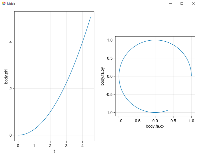
fig = Figure()

ax1 = Axis(fig[1, 1], xlabel="t", ylabel="body.phi")
lines!(ax1, sol.t, sol[body.phi])

ax2 = Axis(fig[1, 2], xlabel="body.fa.ox", ylabel="body.fa.oy", aspect=DataAspect())
lines!(ax2, sol[body.fa.ox], sol[body.fa.oy])

display(fig)

generated figure

[ChrisRackauckas]

Is this initialization? This seems like a state priority / dummy derivative thing? @YingboMa