DifferentialEquations.jl
 DifferentialEquations.jl copied to clipboard
SavedValues not stored at events
DifferentialEquations supports storing additional values (besides u, du) at a pre-defined time-grid. However, it seems not possible to store additional values also at event points. Note, this is important for typical physical systems as simulated by Modia. Assume for example to simulate the following electrical circuit with an ideal switch that is opened and closed at pre-defined time instants:
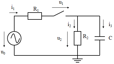
This system has one state (u2, the voltage drop of the capacitor C; so u = [u2]) and it is possible to transform this circuit to one differential equation with this state and compute all other variables explicitly as function of u2 (so u0, i1, u1, i2, i3). The goal would be to simulate this circuit with an ODE integrator of DifferentialEquations and store and plot all variables of this electrical circuit at the given communication time grid and also at events (whenever the switch opens and closes an event is triggered). I do not see, how this can be formulated with DifferentialEquations. A (very bad) workaround is to formulate this system as DAE and have u = [u2, u0, i1, u1, i2, i3] (an ODE integrator can no longer be used and the DAE system is unnecessarily large; for larger physical systems of this type, especially mechanical systems, the DAE-size would become excessive).
In order to test this concretely, here is a simple bouncing ball model where one additional variable is stored additionally:
module Test_bouncingBall3

using DifferentialEquations, PyPlot

function f(du,u,p,t)
  du[1] = u[2]
  du[2] = -9.81
end

function outputs(u, t, integrator) # called at communication points
    return 0.5*u[1]
end

function condition(u,t,integrator) # Event when event_f(u,t) == 0
 z = u[1] + 1e-12
 return z
end

function affect_neg(integrator)
  integrator.u[2] = -0.8*integrator.u[2]
end

u0 = [1.0,0.0]
tspan = (0.0,3.0)

t_start = 0.0
t_inc   = 0.01
t_end   = 3.0
tspan   = (t_start, t_end)
tspan2  = t_start:t_inc:t_end

saved_values=SavedValues(Float64, Float64)
cb1 = SavingCallback(outputs, saved_values, saveat=tspan2)
cb2 = ContinuousCallback(condition,nothing,affect_neg! = affect_neg)

prob = ODEProblem(f,u0,tspan)
sol = solve(prob,Tsit5(),saveat=t_inc,callback=CallbackSet(cb1,cb2))

figure(1)
clf()
plot(sol.t, getindex.(sol.u, 1), label="h")
plot(saved_values.t, saved_values.saveval, label="outputs")
grid(true)
legend()

println("length(sol.t)          = ", length(sol.t))
println("length(saved_values.t) = ", length(saved_values.t))
end
Executing this model results in:
length(sol.t)          = 313
length(saved_values.t) = 301
so the time vector for u and for saved_values is different (because no additional variables are stored at event points).
A temporary work-around is to organize the storing of results in the following way:
- The default storing of "u" in "sol" is switched off (store only first and last point)
- The results are stored in an own datastructure that resides in "p" (in order to be available in "sol") in the following way:
- FunctionCallingCallback callback stores variables at communication points
- With affect! callback the variables before the event are stored at the beginning of the function and the variables after the event at the end of the function.