PhysX
 PhysX copied to clipboard
PhysX Integration Scheme
Hello Devs,
I have a question on how exactly the equations of motion are solved by PhysX. The reason I'm interested in these details is a comparison between Matlab and the Games Engine Unity for robotics applications. To better understand the deviations it is important to understand the underlying algorithms and methods of the program for later evaluation.
One answer I got (https://github.com/NVIDIAGameWorks/PhysX/issues/422) explained that PhysX uses the backward Euler scheme and a constraint based approach. This makes sense for contacts and hard limits were a linear complementarity problem (LCP) can be defined and solved by an iterative solver (PGS or TGS). Another answer I got on the NVIDIA forum (https://forums.developer.nvidia.com/t/damping-of-a-revolute-joint/176867/7) describes an explicit scheme to calculate the new positions and velocities.
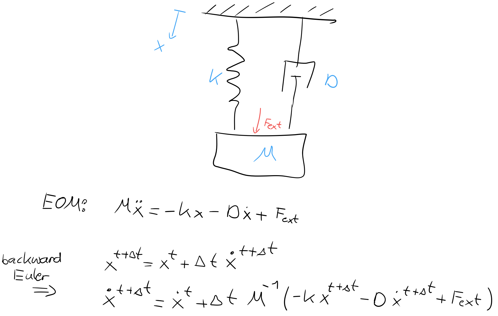
Now my question is how exactly I can formulate a LCP out of the equations of motion discretized using a backward Euler scheme, i.e. which complementary condition to use for the LCP. If possible please explain the approach based on the simple spring-damper system shown in the Figure.
In case the explicit Euler scheme is used, which role plays the PGS or TGS solver?
Thanks in advance! Kind regards, Niklas
Often the devs are quite repsonsive here so hopefully someone more knowledgeable than me can help you out but...
The docs say: "Springs are fully implicit: that is, the force or acceleration is a function of the position and velocity after the solve."
I believe this agrees with the response you got on your forum post: "The integration scheme for the joint drives is implicit. In particular, the force applied by the drive is constant over a time step, but it is computed from the projected end-of-timestep joint state given the applied force and response of the joint at the beginning of the timestep."
If you're feeling adventurous you could look at https://github.com/NVIDIAGameWorks/PhysX/blob/c3d5537bdebd6f5cd82fcaf87474b838fe6fd5fa/physx/source/lowleveldynamics/src/DySolverConstraint1D.h#L177 and the calling code. I believe this is effectively where the magic happens for a simple (non featherstone) spring damper.
Someone I once worked with who knew a lot more about numerical methods than me once mentioned that explicit schemes tend towards overshoot (i.e. gain of energy) whereas implicit schemes tend towards undershoot (loss of energy). This might explain why your implicit unity solution appears so much more damped than your explicit matlab solution. The wiki article of backward euler (https://en.wikipedia.org/wiki/Backward_Euler_method) has an analysis section which might be saying the same thing. I don't know how to interpret it but maybe you do and it will confirm what I'm saying. In either case the error will be a function of the timestep so it's unsurprising that the two solutions were closer when you reduced the timestep.
Thank you for the reply!
Your comments are correct I misinterpreted the message in the Nvidia forum. I tried to apply the approach to the spring-damper system and got the following:
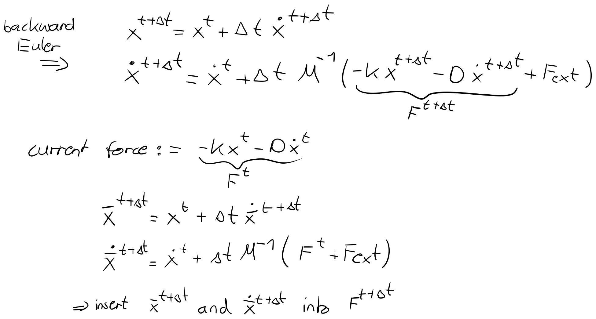 I basically compute an intermediate velocity and position to insert them in the equation for the velocity/position of the next timestep. It is still unclear to me where exactly the iterative solver is needed in this approach. This would be important for my experiments because the PGS and TGS solver produce different solutions.
I'll try to understand the code but in the past that seemed to be a hopeless path. This simple spring-damper system should only function as a reference to better understand the underlying approach for articulated bodies, which use featherstones algorithm.
It is correct that explicit schemes tend to overshoot (i.e. pump energy into the system) and implicit schemes tend to undershoot (i.e. dissipation of energy). Thinking about PhysX it makes sense that an implicit scheme is used to ensure stability. This would also explain the additional damping in my experiments discussed in the Nvidia forum.
I'm asking for these detailed information to identify the source of the remaining errors in the Unity simulation. These errors are explained in another issue: https://github.com/NVIDIAGameWorks/PhysX/issues/434.
I'd like to help you more but I don't think I can. It does seem to me that the implicit equations can be solved algebraically for a simple spring-damper. Perhaps the iteration is to compensate for the fact that it's a multibody, multiconstraint system so there's a lot more interdependent variables in the general case than in this simple example.
Hi Niklas,
The equations you have for backward Euler look correct to me, so you should be able to predict the PGS results using these equations. You could test with a simple revolute joint drive and a single link (the drive is like a spring damper).
For TGS, the results will vary with the number of iterations. TGS will subdivide the timestep into dt / pos_iterations, and then apply a single PGS pos iteration per subdivision. Without contacts, one step is just one backward Euler step.
So you can get the TGS behavior with pos_iterations PGS steps at dt / pos_iterations. Use zero velocity iterations for the comparison. And make sure you have no other friction as well (joint friction or link rigid-body damping).
Finally, you could analyze the effect of the time-step subdivision on the effective discrete-time control gains (i.e. stiffness and damping) to explain the different dynamics.
Hope this helps. Philipp
Hello Philipp,
thanks a lot for the reply. Your answer confirms the knowledge I already gathered about the TGS solver.
One important piece is still missing for my own understanding of the approach in PhysX. The PGS is an iterative solver and I still don't quite get which value is computed using this algorithm. For hard constraints the method is clear to me because a hard condition can be defined: "The velocity at the contact is 0". Afterwards the PGS solver can compute the needed force to ensure this constraint and the new velocity and position can be computed with the equations above.
The mentioned approach is based on the book "Physics-based Animation" by Kenny Erleben. The discretized equations of motion are defined as:
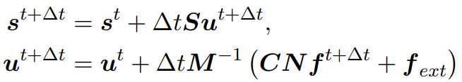 Until here the approach is identical to the simple example above. Formulating the following contact condition
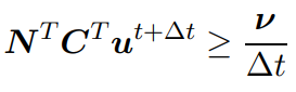 results in the linear complementarity problem for the contact forces after substituting u^(t+dt):
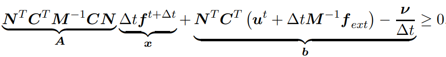
The basic principle of the approach should be explained by these equations. Now the main question is how to formulate a LCP "Ax-b=0" for soft limits i.e. a spring-damper system?
Thanks a lot in advance!
I am not sure I understand your question. A soft limit is continuous, so it does not make sense to formulate it with an LCP I think. I.e. there is a force generated no matter what the constraint distance, i.e. the spring deflection is.
More details on the TGS solver are here, which may be helpful: https://matthias-research.github.io/pages/publications/smallsteps.pdf
That's exactly my point. What equation does the iterative solver solve when no LCP is formulated. My experiments have shown that the results vary for PGS or TGS even for a single revolute joint without friction. If the equations, like those shown for the spring-damper system, are used the solution can directly be computed without the need of an iterative solver.
As @asdasdasdasdasdf mentioned earlier the equations for the spring-damper model can be solved algebraically but the PGS solver might be needed for a multibody system. I'm interested in the equations that are used by the PGS solver and the values that are returned by the solver.
Let me rephrase my previous question: Where exactly comes the PGS solver to play when no collisions and friction are present and only the spring-damper system of a single revolute joint needs to be solved? Additionally it would be interesting what is changed for a kinematic chain with multiple revolute joints.
If there are no collisions or other constraints, the solver will just do the backward euler step I mentioned above. The differences between TGS and PGS should be due to the subdivision of the timestep, i.e. doing a single backward euler vs. multiple. You can try the multi-PGS stepping I suggested above to see if you get the same results.
I think my problem lies in the iterative character of the solver. If i understood correctly, during on timestep delta_t, the PGS solver computes k iterations to get the new position and velocity. The TGS introduces n substeps delta_t/n during which k=1 solver iteration is performed. Is that correct?
Just to be sure i formulated the iterative equations for the above test case:
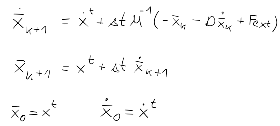 The start values for the PGS solver are position/velocity at timestep t and after k iterations of equations in the picture the position/velocity at time 1+delta_t are computed using the equations of my initial comment.
Again, the TGS solver would use only one iterations of the presented equations for each substep delta_t/n.
Iterating with the drive solver is for the purpose of making it capable of solving multi-body problems correctly.
Putting a spring model into an iterative solver requires changing the way we format the spring. An explicit or implicit spring is simple enough to implement. However, if you repeatedly solve a simple spring formula inside an iterative solver, it will eventually converge on a hard constraint given enough iterations. A softer spring will require more iterations to converge on a hard constraint, but it will get there eventually.
The implicit spring formula PhysX uses converts the spring stiffness into some implicit parameters, which are the "velMultiplier", "bias" and "impulseMultiplier".
As the spring becomes stiffer/damping becomes larger, velMultiplier converges on the -(effective mass), impulse Multiplier converges on 1 and constant converges on the velocity/integrated positional error terms multiplier by the effective mass. This means that setting stiffness or damping terms very large converges on a hard constraint rather than becoming numerically unstable. Where the spring coefficients do not converge on a hard constraint, the correct spring-like behavior should be observed because the forces that have been applied in previous iterations are recorded and fed into the implicit spring solver each iteration so the spring itself will not produce stiffer/more damped behavior than expected.
In a simple 2-body/1 spring problem, the first solver iteration will produce the full force required by the spring to satisfy the constraint and any subsequent iterations will apply zero force.
When there are multiple constraints/bodies involved, multiple iterations may apply forces because the solver is converging on an answer for a multi-body problem without knowing the total effective mass of the systems attached at each end of the spring. The individual spring formula only considered the mass of the individual bodies that are directly connected.
The Featherstone articulation model uses a similar spring model for its drives, with the exception that the total mass of the system either side of the spring is considered. In this case, the spring drive can be solved correctly in far fewer iterations, although you may still need more than 1 iteration if there are multiple springs, contacts and joint limits involved.
If you would like to see where these parameters are set up, search for "setSolverConstants" in DySolverConstrant1D.h.
Thanks a lot for the answer!
Based on your comment I got some new questions:
I don't understand what you mean by the hard constraint when solving a spring equation iteratively. And why exactly is that a problem?
For a large stiffness/damping a hard constraint is reached. This means the spring acts like a "wall" and perfoms no deformation any more. Previous in your comment this seemed to be a problem but now it is desireable to keep the solver stable.
Maybe we can discuss the 2-body/1 spring problem in more detail. As i understood it the first solver iteration applies the spring force using the position at the timestep t. Which euations do the subsequent iterations solve?
Regarding robotics simulation the case of the Featherstone articulation model is most important for my experiments. Could you please explain to my the basic steps PhysX takes to solve such a system. I would really appreciate it to know which equations the iterative solver uses and which variables are computed by the solver. Additionally I'm interested in the termination criterion of the solver, i.e. which parameter should be minimized.
In general I would like to understand the basic approach PhysX uses to compute the dynamics of an articulated body. During my research I understood the Featherstone algorithm and the Constraint-based approach to solve contacts and hard limits. Right now the most important part, computing the dynamics of an articulated body, is still missing. In case my questions are to detailed could you please redirect me to some sources the solver of PhysX is based on so I can understand the low level approach?
Converging on a hard constraint rather than becoming unstable when the stiffness/damping coefficients of the drive are set very high is often a desirable property for a simulator.
Incrementally converging on a hard constraint when the coefficients used should have yielded a soft constraint as you run more iterations is an undesirable property. This introduces an unwanted relationship between iteration count and behavior. While the behavior will often be influenced by the iteration count, the intention is that more iterations should converge on a more correct result.
Consider that you run a spring simulation based on the current positional and velocity state of your bodies and apply those forces to the respective bodies N times in a single frame; you would not want this to result in a force that was N times larger than the analytically-expected force.
With the PhysX iterative spring model, subsequent iterations use the same spring parameters as the first iteration, with the key difference being that the velocity state of the bodies has changed and the accumulated applied force changes from iteration to iteration. The solver uses a scaled accumulation of the previously applied force (scale based on impulseMultiplier), added to the spring formula based on the current velocity/positional state to define the total required force from the spring based on the state in that iteration. The (unscaled) previously-applied force is then subtracted from the total required force to determine how much force to apply this given iteration. The previously applied force starts at zero and is accumulated each iteration. This ensures in single-joint cases that the correct force is calculated in a single iteration, while subsequent iterations apply zero force.
So the solver adds a small spring force each iteration until an equilibrium with the weight force of the mass and other external forces is reached?