Integrating AdvancedHMC

[xukai92]

I'd like to give a try on integrating Poriot with AdvancedHMC when I find some time. Can you give me some brief intro of how it should be done?

[MikeInnes]

using Poirot, IRTools

coin() = rand(Bool)

f = () -> begin
  a = coin()
  b = coin()
  observe(a | b)
  a & b
end

Get a trace / static graph for the generative model:

julia> ir = Poirot.trace(typeof(f))
1: (%1 :: var"#9#10")
  %2 = (rand)(Bernoulli{Rational{Int64}}(p=1//2)) :: Bool
  %3 = (rand)(Bernoulli{Rational{Int64}}(p=1//2)) :: Bool
  %4 = (|)(%2, %3) :: Bool
  %5 = (Poirot.observe)(%4) :: Nothing
  %6 = (&)(%2, %3) :: Bool
  return %6

Transform this into a logpdf, along with a list of random variables and their types:

julia> lpdf, vars = Poirot.logprob(ir);

julia> vars
2-element Array{Any,1}:
 (%2, Bool)
 (%3, Bool)

Transform this into an executable Julia function and run it (it returns both the result of the infer block and a log probability for that result):

julia> lpdf = IRTools.func(lpdf)
##254 (generic function with 1 method)

julia> lpdf(nothing, (true, false))
(false, -1.3862943611198906)

julia> lpdf(nothing, (false, false))
(false, -Inf)

You should be able to treat lpdf as a normal function, including differentiating with Zygote to get a gradient. I believe that's all you need for HMC but let me know if there's something else.

[xukai92]

Somehow came across this old issue and play with Poirot a bit today. I managed to make a model with discrete observations work with HMC---see below.

sigmoid(x) = 1 / (1 + exp(-x))

f = () -> begin
    l = randn()
    p = sigmoid(l)
    
    a = rand(Bernoulli(p))
    b = rand(Bernoulli(p))
    c = rand(Bernoulli(p))
end

ir = Poirot.trace(typeof(f))
_lpdf, vars = Poirot.logprob(ir)
_lpdf = IRTools.func(_lpdf)

lpdf = x -> _lpdf(nothing, (x[1], true, true, false))[2] # observations are a=true, b=true, c=false
gpdf = x -> only(Zygote.gradient(lpdf, x))

using AdvancedHMC, ForwardDiff

dim = 1
xinit = randn(dim)

n_samples = 2_000

metric = DiagEuclideanMetric(dim)
hamiltonian = Hamiltonian(metric, lpdf, ForwardDiff)

integrator = Leapfrog(0.5)
proposal = NUTS{MultinomialTS, GeneralisedNoUTurn}(integrator)

samples, stats = sample(hamiltonian, proposal, xinit, n_samples; verbose=false)

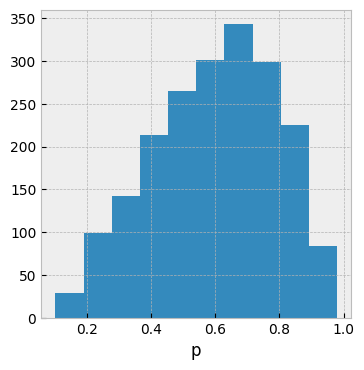
The sample histogram looks correct to me:

In the meanwhile, I don't know how to make a simple model with continuous observation work, e.g. below fails by not moving at all in the sampling

f = () -> begin
    m = randn()
    
    x = rand(Normal(m, 1))
end

# ...

lpdf = x -> _lpdf(nothing, (x[1], 1.0))[2]

but I'd expect to sample m around 1.0.