DFTK.jl
 DFTK.jl copied to clipboard
Comparison of DFTK vs QE for magnetic PrNiO3
This is a test case of a larger 20 atom unit cell with slight disproportionation (low symmetry) and magnetism.
The difference in performance is quite dramatic, QE runs in about 5-10s per scf step, DFTK on the order of 6 min. Tested on a 14 core recent intel workstation, Threads.nthreads() = 14. QE was ran with 14 mpi processes and compiled with intel compilers and mkl.
DFTK input:
using DFTK
using UnitfulAtomic
using Unitful
using Unitful: Å

lattice = uconvert.(UnitfulAtomic.bohr, [5.44051478455355Å -3.246834533897242e-8Å -0.029786855045508258Å;
                                        -5.95252997881161e-8Å 5.423764532946292Å 2.164556355931495e-8Å;
                                        -0.014091088712605556Å 5.4113908898287375e-9Å 7.665287350427802Å])

Ni_atpos = [[0.0, 0.0, 0.0],
            [0.5, 0.50001, 0.5],
            [0.49999, 0.50001, 1.0e-5],
            [-1.0e-5, -1.0e-5, 0.50001]]

O_atpos = [[0.57391, 0.49048, 0.26118],
           [0.92609, 0.99049, 0.23883],
           [0.42609, 0.50951, 0.73883],
           [0.07392, 0.00952, 0.76118],
           [0.20659, 0.27242, 0.04079],
           [0.2934, 0.77242, 0.4592],
           [0.7934, 0.72758, 0.9592],
           [0.70659, 0.22758, 0.54079],
           [0.73053, 0.20897, 0.95945],
           [0.76947, 0.709, 0.54056],
           [0.26947, 0.791, 0.04056],
           [0.23053, 0.29103, 0.45945]]

Pr_atpos = [[0.49167, 0.03805, 0.25047],
            [0.00834, 0.53804, 0.24953],
            [0.50834, 0.96196, 0.74953],
            [0.99167, 0.46195, 0.75047]]


Ni = ElementPsp(:Ni, psp=load_psp("hgh/lda/ni-q18.hgh"))
O  = ElementPsp(:O, psp=load_psp("hgh/lda/o-q6.hgh"))
Pr = ElementPsp(:Pr, psp=load_psp("hgh/lda/pr-q13.hgh"))

atoms = [Ni => Ni_atpos, O => O_atpos, Pr => Pr_atpos]
Ni_magmom = [0,0,2.0,-2.0]
O_magmom = zeros(length(O_atpos))
Pr_magmom = zeros(length(Pr_atpos))

Ecut = 45/2
kgrid = [4, 4, 2]
mag_moms = [Ni => Ni_magmom, O => O_magmom, Pr => Pr_magmom]
model_afm = model_LDA(lattice, atoms, magnetic_moments=mag_moms, temperature=0.001)

basis = PlaneWaveBasis(model_afm, Ecut;kgrid=kgrid)

ρ0=guess_density(basis, mag_moms)

scfres = self_consistent_field(basis, tol=1e-6, ρ=ρ0, mixing=KerkerMixing())
QE 6.7 develop scf input:
&control
  prefix = 'PrNiO3'
  verbosity = 'high'
  calculation = 'scf'
  outdir = './outputs'
  pseudo_dir = '/home/lponet/Documents/occupations/PrNiO3/'
  restart_mode = 'from_scratch'
/

&system
  ibrav = 0
  nat = 20
  ntyp = 7
  ecutwfc = 50.0
  starting_magnetization(2) = 1.0
  starting_magnetization(3) = -1.0
  occupations = 'smearing'
  nspin = 2
  smearing = 'gaussian'
  degauss = 0.001
/

&electrons
  mixing_beta = 0.2
  electron_maxstep = 200
  conv_thr = 0.0001
  mixing_mode = 'local-TF'
/

ATOMIC_SPECIES
Ni3 58.6934   Ni.upf
Ni1 58.6934   Ni.upf
Ni2 58.6934   Ni.upf
O1 15.9994   O.upf
O2 15.9994   O.upf
O3 15.9994   O.upf
Pr 140.9077   Pr.pbesol_ps.uspp.UPF

CELL_PARAMETERS (angstrom)
5.44051478455355 -5.95252997881161e-8 -0.014091088712605556
-3.246834533897242e-8 5.423764532946292 5.4113908898287375e-9
-0.029786855045508258 2.164556355931495e-8 7.665287350427802

ATOMIC_POSITIONS (crystal)
Ni3  0.0 0.0 0.0
Ni3  0.5 0.50001 0.5
Ni1  0.49999 0.50001 1.0e-5
Ni2  -1.0e-5 -1.0e-5 0.50001
O1  0.57391 0.49048 0.26118
O1  0.92609 0.99049 0.23883
O1  0.42609 0.50951 0.73883
O1  0.07392 0.00952 0.76118
O2  0.20659 0.27242 0.04079
O2  0.2934 0.77242 0.4592
O2  0.7934 0.72758 0.9592
O2  0.70659 0.22758 0.54079
O3  0.73053 0.20897 0.95945
O3  0.76947 0.709 0.54056
O3  0.26947 0.791 0.04056
O3  0.23053 0.29103 0.45945
Pr  0.49167 0.03805 0.25047
Pr  0.00834 0.53804 0.24953
Pr  0.50834 0.96196 0.74953
Pr  0.99167 0.46195 0.75047

K_POINTS (automatic)
 4 4 2 0 0 0
If I made a stupid mistake, please let me know and I can retry!
Cheers!
From a quick profile there doesn't seem to be any obvious wasted time. I find it hard to believe that QE does the same thing in 5s, even with threading.
- Can you check if QE uses symmetries? DFTK doesn't detect any here.
- Can you check QE uses the same number of electrons in the pseudos?
Hi and thanks for this report. Modulo the threading / parallelisation aspect, I also find it hard to think of a place we would be loosing a lot of time over QE. What came to my mind is:
The mixing settings are not identical (local-TF with 0.2 damping in QE versus plain Kerker with default 0.8 damping in DFTK). Also in QE you seem to converge the SCF less tightly. Do you have the respective number of SCF iterations in both codes?
Minor point (probably not so revelant): The smearing also differs. We use Fermi-Dirac by default.
Also we apply a kshift by default if the kpoint grid is even, so the BZ sampling differs in QE and DFTK (and thus likely the symmetries). Try kshift=[0,0,0] in the PlaneWaveBasis construction.
Mixing is probably irrelevant if he's comparing time per SCF. Kpoint sampling might be important though (more or less symmetry reduction depending on kpoint shift)
Ah sorry I overread that. I'd still be interested in the number of SCF steps though ;)
kshift didn't change much.
The QE pseudos:
Ni: US, pbesol, z valence = 18, 3s 3p 3d 4s 4p
O: PAW, pbesol, z valence = 6, 2s 2p 3d
Pr: US, pbesol, z valence = 11, 5s 5p 5d 6s 6p
Convergence seems to be achieved in less steps than with QE though.
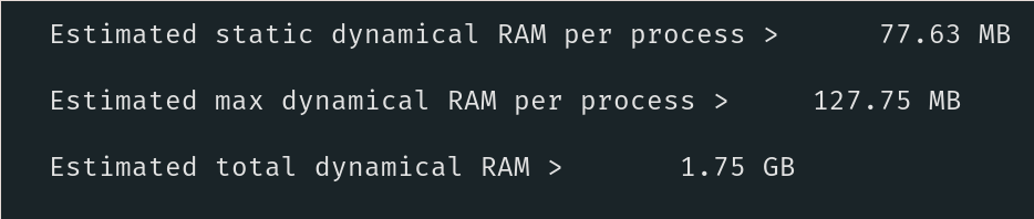
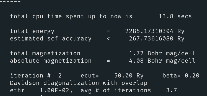
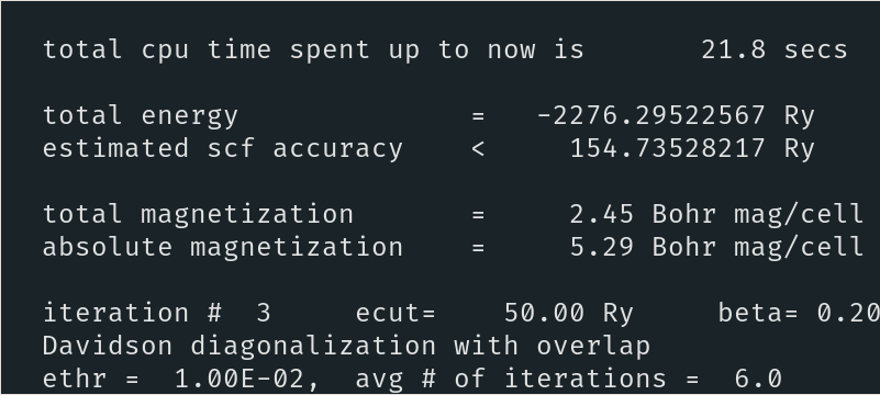
QE Doesn't detect any symmetries either. Also the memory usage is quite different. I've attached some screenshots of QE:
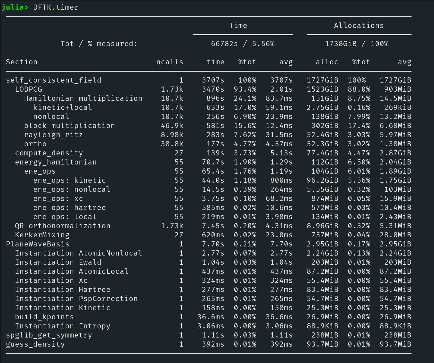
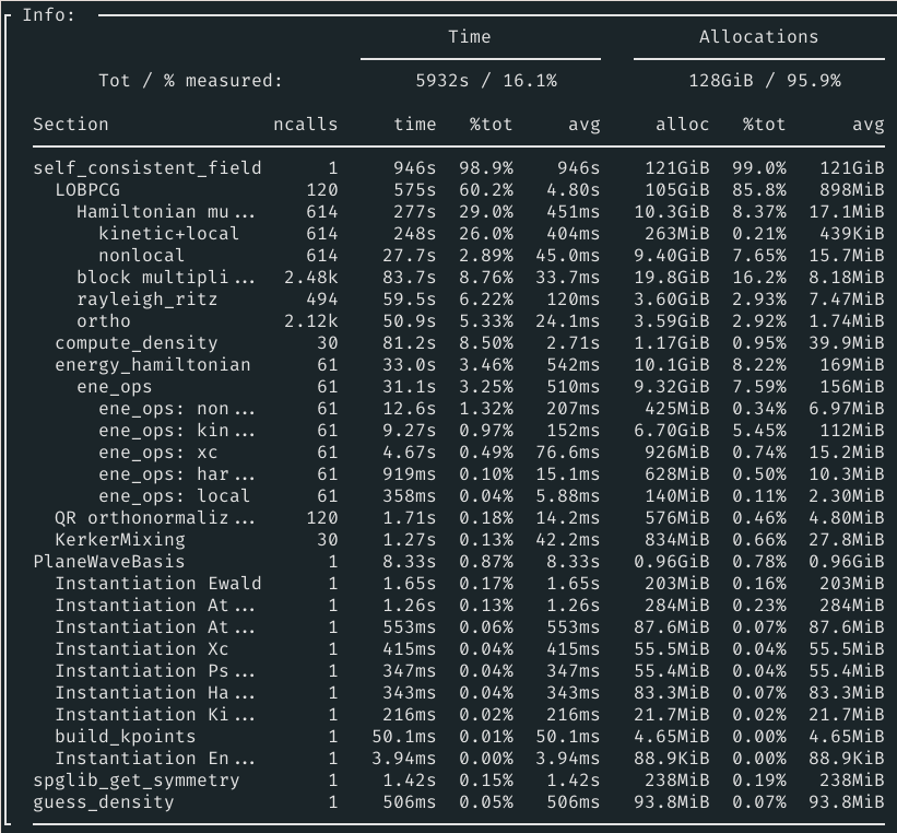
DFTK Timing output after run finished:
Weird. Can you post as a gist the output of both DFTK and QE? @mfherbst are you able to use your magical converter tools to make sure both inputs roughly match?
I'll try to give it a go tomorrow. Would be good to have input and output of both codes in plain text, if possible @louisponet.
well, inputs are in the first post, output for scf is: scf.out
The dftk output (DFTK convergence is much nicer than QE):
n     Free energy       Eₙ-Eₙ₋₁     ρout-ρin   Magnet   Diag
---   ---------------   ---------   --------   ------   ----
  1   -946.8751582930         NaN   7.04e+00   -0.001    13.4
Diagonalising Hamiltonian kblocks: 100%|███████████████████████████████████████████████████████████████| Time: 0:04:44
  2   -940.5413766477    6.33e+00   4.12e+00   -0.000    14.7
Diagonalising Hamiltonian kblocks: 100%|███████████████████████████████████████████████████████████████| Time: 0:04:42
  3   -990.0552472211   -4.95e+01   2.06e+00   -0.000    10.9
Diagonalising Hamiltonian kblocks: 100%|███████████████████████████████████████████████████████████████| Time: 0:04:46
  4   -1008.616714451   -1.86e+01   4.87e-01   -0.000    15.5
Diagonalising Hamiltonian kblocks: 100%|███████████████████████████████████████████████████████████████| Time: 0:03:17
  5   -1008.644052804   -2.73e-02   6.28e-01   -0.000    10.2
Diagonalising Hamiltonian kblocks: 100%|███████████████████████████████████████████████████████████████| Time: 0:02:00
  6   -1009.775140349   -1.13e+00   3.52e-01   -0.000    3.3
Diagonalising Hamiltonian kblocks: 100%|███████████████████████████████████████████████████████████████| Time: 0:02:07
  7   -1009.634491636    1.41e-01   2.54e-01    0.000    2.2
Diagonalising Hamiltonian kblocks: 100%|███████████████████████████████████████████████████████████████| Time: 0:03:05
  8   -1009.055705098    5.79e-01   3.98e-01   -0.000    8.2
Diagonalising Hamiltonian kblocks: 100%|███████████████████████████████████████████████████████████████| Time: 0:01:44
  9   -1010.024935944   -9.69e-01   8.07e-02   -0.001    2.3
Diagonalising Hamiltonian kblocks: 100%|███████████████████████████████████████████████████████████████| Time: 0:01:22
 10   -1010.038962296   -1.40e-02   7.26e-02   -0.002    1.9
Diagonalising Hamiltonian kblocks: 100%|███████████████████████████████████████████████████████████████| Time: 0:01:17
 11   -1010.022739976    1.62e-02   8.39e-02   -0.003    1.0
Diagonalising Hamiltonian kblocks: 100%|███████████████████████████████████████████████████████████████| Time: 0:01:17
 12   -1010.057141994   -3.44e-02   4.42e-02   -0.002    1.0
Diagonalising Hamiltonian kblocks: 100%|███████████████████████████████████████████████████████████████| Time: 0:01:18
 13   -1010.068263132   -1.11e-02   1.51e-02   -0.000    1.0
Diagonalising Hamiltonian kblocks: 100%|███████████████████████████████████████████████████████████████| Time: 0:02:12
 14   -1010.061265174    7.00e-03   3.31e-02   -0.002    6.9
Diagonalising Hamiltonian kblocks: 100%|███████████████████████████████████████████████████████████████| Time: 0:01:27
 15   -1010.068680111   -7.41e-03   1.08e-02   -0.000    2.0
Diagonalising Hamiltonian kblocks: 100%|███████████████████████████████████████████████████████████████| Time: 0:01:16
 16   -1010.069063860   -3.84e-04   7.81e-03   -0.001    1.2
Diagonalising Hamiltonian kblocks: 100%|███████████████████████████████████████████████████████████████| Time: 0:01:17
 17   -1010.069386480   -3.23e-04   2.65e-03   -0.000    1.1
Diagonalising Hamiltonian kblocks: 100%|███████████████████████████████████████████████████████████████| Time: 0:02:05
 18   -1010.069406701   -2.02e-05   1.37e-03   -0.000    9.2
Diagonalising Hamiltonian kblocks: 100%|███████████████████████████████████████████████████████████████| Time: 0:02:16
 19   -1010.069369457    3.72e-05   2.51e-03   -0.000    7.1
Diagonalising Hamiltonian kblocks: 100%|███████████████████████████████████████████████████████████████| Time: 0:01:43
 20   -1010.069376218   -6.76e-06   2.45e-03   -0.000    2.3
Diagonalising Hamiltonian kblocks: 100%|███████████████████████████████████████████████████████████████| Time: 0:01:47
 21   -1010.069374751    1.47e-06   2.30e-03   -0.000    2.2
Diagonalising Hamiltonian kblocks: 100%|███████████████████████████████████████████████████████████████| Time: 0:01:48
 22   -1010.069341602    3.31e-05   3.31e-03   -0.000    2.3
Diagonalising Hamiltonian kblocks: 100%|███████████████████████████████████████████████████████████████| Time: 0:01:53
 23   -1010.069365532   -2.39e-05   2.70e-03   -0.000    2.6
Diagonalising Hamiltonian kblocks: 100%|███████████████████████████████████████████████████████████████| Time: 0:01:43
 24   -1010.069407416   -4.19e-05   1.10e-03   -0.000    1.9
Diagonalising Hamiltonian kblocks: 100%|███████████████████████████████████████████████████████████████| Time: 0:01:18
 25   -1010.069408805   -1.39e-06   8.76e-04   -0.000    1.7
Diagonalising Hamiltonian kblocks: 100%|███████████████████████████████████████████████████████████████| Time: 0:01:17
 26   -1010.069398073    1.07e-05   1.42e-03   -0.000    1.0
Diagonalising Hamiltonian kblocks: 100%|███████████████████████████████████████████████████████████████| Time: 0:01:18
 27   -1010.069405907   -7.83e-06   1.07e-03   -0.000    1.0
Diagonalising Hamiltonian kblocks: 100%|███████████████████████████████████████████████████████████████| Time: 0:01:17
 28   -1010.069411470   -5.56e-06   4.81e-04   -0.000    1.0
Diagonalising Hamiltonian kblocks: 100%|███████████████████████████████████████████████████████████████| Time: 0:01:17
 29   -1010.069407791    3.68e-06   8.63e-04   -0.000    1.1
Diagonalising Hamiltonian kblocks: 100%|███████████████████████████████████████████████████████████████| Time: 0:01:17
 30   -1010.069410581   -2.79e-06   6.13e-04   -0.000    1.2
Diagonalising Hamiltonian kblocks: 100%|███████████████████████████████████████████████████████████████| Time: 0:01:17
 31   -1010.069411736   -1.15e-06   4.45e-04   -0.000    1.0
Diagonalising Hamiltonian kblocks: 100%|███████████████████████████████████████████████████████████████| Time: 0:01:18
 32   -1010.069411975   -2.39e-07   3.46e-04   -0.000    1.0
OK so from a cursory inspection:
- It seems QE is using LDA+U; we don't support this. There should be no significant impact on perf, but it might explain why the results are different
- We are using a similar number of hamiltonian application per SCF, so timings should be comparable there
- QE is run under MPI. Can you either run QE without MPI, or run DFTK with MPI? See https://juliamolsim.github.io/DFTK.jl/dev/guide/parallelization/. We only support MPI over kpoints for now, which should be relatively performant here. I'm not sure what distribution QE takes
- We have 32 kpoints. QE uses time reversal symmetry (which we don't yet support) and so has 20 kpoints.
- We actually have a slightly smaller FFT grid; this is probably because you used 45 Ry in DFTK and 50 in QE; you can check this with basis.fft_size.
- We have 196 valence electrons (model.n_electrons), QE has 188. This is because QE's Pr psp has 11 electrons, we have 13. QE ends up using 113 "kohn-sham states", although I'm not sure how it gets there...
Re the last point, I'm guessing from https://lists.quantum-espresso.org/pipermail/users/2012-December/026012.html, that that would be 113*2 states in total. We do something similar, so there should be no large discrepancy there.
it might explain why the results are different
... and why our SCF converges faster. The collinear cases are usually much easier to converge
We do something similar, so there should be no large discrepancy there.
Yes, I "stole" the 20% extra from QE.
OK, so at a very rough level it would seem based on the above that QE should be about 2x faster than DFTK for a serial run (because of better kpoint reduction, and slightly less electrons). Throwing an extra factor of 10x to account for parallelization (to be checked by running DFTK with MPI), that accounts for a factor of 20x. That still leaves a factor 3x, which is weird, but we should check this more carefully by making a more fair comparison: using same pseudos and Ecut, not using LDA+U, disabling time-reversal in QE - "noinv=false", and using the same parallelization scheme (MPI in both cases).
We should also get around to supporting TRS (https://github.com/JuliaMolSim/DFTK.jl/issues/224). That's not particularly hard, but fiddling with symmetries is always annoying.
I ran QE with the noinv = true, leading to the full 32 kpoints, but together with the lower cutoff of 45 it is pretty much the same as before. Sidenote, QE actually doesn't really converge well even without +U, probably because a denser k-grid would be needed.
DFTK output with mpirun -n 14:
I think 31.5s yes, The difference seems to be mainly in the first couple of iterations where DFTK does a lot more iterations to get the Hami diagonalized (18ish vs 4ish in QE). But indeed it's not far off.
OK cool! We have selected relatively stringent convergence criteria for increased robustness so I'm comfortable if the difference is purely attributable to that.
Okay so idk if it's a valid way of comparing, but if I take the mean seconds/diag iteration I get 2.433s in QE and 6.446s in DFTK. So it's not purely the additional amount of diagonalization iterations. But the difference is also not enormous, which is great. So QE uses davidson, and I think scalapack to do the BLAS operations, probably having all of that compiled using intel compilers etc could already explain part of it. Maybe the additional allocations that seem to be happening in DFTK another part?
That seems fair. Possibly we do at least two hamiltonian applications even when we say 1, which could explain a bit of it. You can probably shave off a bit of time by using MKL (which if I understand correctly in recent versions of julia is as simple as doing a Pkg.add). Allocations I don't think are that big of an effect...
Yes I just checked, we do a hamiltonian application to compute the residual, and another to compute A on the residuals to be able to do the Rayleigh-Ritz. So even if we report 1 iteration it means two hamiltonian applications. Summoning here @haampie because I seem to vaguely remember he told me QE had a way of avoiding this
Yeah, QE does not apply the Hamiltonian when it computes residuals, it stores all basis vectors ϕ together with Hϕ and Sϕ applied to them. Also it may not even compute residual norms, but base the convergence criterium on the change in the Ritz values; that avoids inner products.
Ah yes that's the change in Ritz value trick I meant, sorry I misremembered. But I guess QE still has to make at least two matvecs per eigenvector to make any progress, right?
But indeed it's not far off.
Also happy that we arrive to that conclusion. Anything else would have worried me quite a bit.
Let me get back to this a in a bit, they can do it with one mat-vec (or let's say, matrix-block-vector) multiplication per expansion step of the davidson method, I can share the pseudo code soon :tm:
@antoine-levitt Didn't we try something like this in the LOBPCG at some point and discarded it, because it led to numerical instabilities, or do I misremember?
@haampie My argument is that for a davidson, even with just one eigenvector, you're going to have to compute r = Ax - lambda_x x, then you update x as x <- alpha x + beta r, where you compute alpha/beta to minimize the Rayleigh quotient, and for that you need to know A r. You could try to fix alpha/beta a priori, and indeed that sometimes works, but it's a bit tricky. And in any case you need to know A r to be able to say anything about the new x.
@mfherbst I don't remember we tried this, but maybe?
These are my notes:
Solve HX = SXΛ approximately, with S pos def, for X = VY where V is the
search space, subject to HX - SXΛ ⟂ V in the S inner product

Low dimensional:
Y  -- pre-ritz vectors (low dimensional)
Λ  -- diag matrix with Ritz vals on the diagonal
and another one to store V'(HV), not named here.

High dimensional:
X  -- ritz vectors
V  -- search space
HV -- H * V
SV -- S * V
HX -- H * X
SX -- S * X
R  -- residual but also used as workspace/tmp storage.

---

Init:
1. Generate initial V
2. Compute (HV) := H * V
3. Compute (SV) := S * V
4. Orthogonalize V, i.e. compute and decompose V'(SV) = LL', and update:
   a. V := VL⁻*,
   b. (HV) := (HV)L⁻*
   c. (SV) := (SV)L⁻*
   so that V'(SV) = I.
5. Solve Galerkin problem: V'(HV)Y = V'(SV)YΛ = YΛ for Y and Λ.

for step = 1, 2, ..., k
    1. if this is not the last iteration (i.e. if we can still expand)
        a. Update these guys -- only for "unconverged" vecs estimated from the change in Ritz values between iterations.
           (HX) := [(HX) (HV) * Y[:, for m selected indices]]
           (SX) := [(SX) (SV) * Y[:, for m selected indices]]
        b. Compute R := (HX) - (SX) * Λ (in the first m cols of R, last m cols of HX and SX, ...)
        c. Compute column-wise norms of R.
        d. Apply preconditioner R := P \ R, and maybe scale for stability.
    2. if we should restart, if everything is converged, or if it's the last iteration
        a. update X := VY -- not necessary if in first iteration (i.e. initial guess was good enough)
        b. if converged or last iteration, break, solution is in X.
        c. otherwise shrink search space,
           (HX) := (HV) * Y[:, first so many indices]
           (SX) := (SV) * Y[:, first so many indices]
           (HV) := (HX)
           (SV) := (SX)
           V := X
    3. Expand! Apply Hamiltonian (on the new block only)
         V  := [V    R    ]     -- just a copy
       (HV) := [(HV) H * R]     -- matmul
       (SV) := [(SV) S * R]     -- matmul
    4. Orthogonalize to old cols. This is the trick where the matrix-vector product is skipped :)
       Notation overloaded, R, (HR) and (SR) refer to the new blocks in V, (HV), (SV),
       and V, (HV) and (SV) refer to those things without thew block.
       a.    R :=  (I - VV'S)R =  R   -   V  * (SR) -- last bit is already computed in last cols of (HV)
       b. (HR) := H(I - VV'S)R = (HR) - (HV) * (SR) -- also, available already!
       c. (SR) := S(I - VV'S)R = (SR) - (SV) * (SR) -- same
    5. Do interior ortho. Again, R, (HR) and (SR) refer to the new block in V, (HV), (SV).
       Decompose R'(SR) = LL'
       a.    R := RL⁻*
       b. (HR) := (HR)L⁻*
       c. (SR) := (SR)L⁻*
    6. Solve Galerkin problem: V'(HV)Y = V'(SV)YΛ = YΛ for Y and Λ. -- you can do a partial solve here!
Which is correct modulo typos and mistakes.
Also this does not do locking, but locking is implemented in SIRIUS (which integrates with QE and adds cuda and rocm support, install through spack using spack install sirius [+cuda cuda_arch=... ^intel-mkl] standalone or as a blackbox solver for QE: spack install q-e-sirius ^sirius +cuda cuda_arch=... ^intel-mkl/^openblas...
Right but that algorithm does nothing (does not update the space spanned by X) if you allow it only one matvec with the hamiltonian, right?
We already do locking, although I'm sure our heuristics could use some tweaking. That might also be a difference wrt QE - possibly QE is faster because of more efficient locking. The right measure here is the total number of matvecs (which we compute and store somewhere)