the formulea for calculating derivatives of different error orders

[thudjx]

Sorry to misuse issues to ask questions, but I could't find any other way to communicate with you developers. I am using this package to calculate the first order derivative of a matrix which can be thought of a function of mono variable x, i.e., M(x). I find that the derivative is hard to converge. By converging I mean if I add more nodes when calculating the derivative, the derivative is unchanged under some tolerance. In practice, I just increase q in central_fdm(q, 1). I have tried q up to 12 but the result didn't seem to convergence. I couldn't increse the order any more because the time for calculation is unacceptable in my case. I also tried to change max_range, and the result is quite different from that calculated with default max_range. That led me to investigate the details of calculating method of FiniteDifferences.jl. I found that the method for calculating derivative in this package is not that easy to understand, especially I find that it choose nodes of two different set.(see picture below) So would you please give some more details on how the nodes are chosen, especially the meaning of max_range and how are the derivatives calculated using the nodes?

[wesselb]

Hey @thudjx!

Would you be able to share the function you're trying to estimate the derivative of?

To answer your questions, max_range specifies the maximum distance from x that the function will be evaluated at. You can use this to deal with singularities or domain issues. The derivatives are computed as a weighted estimate of the function evaluations by eliminating the first q - 1 terms of the Taylor expansion not including the derivative. (Specifically, this happens here.)

To improve the accuracy of the estimate, you have a few knobs that you can play with. (Some of these you have already tried, but I'll include them anyway for completeness.)

• Increase the order q of the method.
• Set max_range to the largest distance from x up to which point the Taylor expansion still converges.
• Change the adaptation of the method, e.g. central_fdm(10, 1, adapt=2). You can set adapt to an integer number to perform so many adaptation steps. You'll generally want to combine higher adapt with a greater max_range. Adaptation means to improve the estimate of the step size by estimating the magnitude of some higher-order derivative using another finite-difference method.
• If that also didn't work, maybe your function is corrupted with (numerical) noise? In that case, you can try setting factor.
• If the above didn't work, try giving a manual step size via fdm = central_fdm(10, 1), fdm(f, x, step). Try a range of step sizes spanning different orders of magnitudes.
• If even that doesn't work, you may have to try something even more fancy like combining FDMs with Richardson extrapolation.

[thudjx]

Thanks for your kind reply! It does help a lot, especically the mensioned factor to deal with the numerical noises.

I have tried different factors for calculating finite differences, and the results seemed much more reasonable than before. But I still can't be sure if I have obtained the correct result, as there is no benchmark for refering.

I have extracted the codes for calculating finite difference from my project and uploaded here. The dependences of functions seem to be deep, but the main function is to calculate the derivative over x of some function of eigenstates of a matrix M(x) which dependents on x.

To sum, my main problem now is how to determine if the obtained derivative has converged. And I would really appreciate it if you could explain more on how the factor parameter eliminates the numerical noice.

[wesselb]

Thanks for uploading the function! I've played around with it, and it seems like a derivative which is really hard to estimate.

To try to get somewhere, I ran a loop comparing, for various orders and manual step sizes, the relative error of derivative(step) and derivative(step / 2):

    for order in [2, 3, 4, 5, 6, 7, 8, 9, 10, 11, 12, 13, 14, 15, 16, 17, 18, 19, 20]
        for step in [1e-6, 1e-7, 1e-8, 1e-9, 1e-10, 1e-11]
            deriv = central_fdm(order, 1, adapt=0)(df, 0, step)
            deriv2 = central_fdm(order, 1, adapt=0)(df, 0, step / 2)
            println("order ", order, " step ", step)
            println("rel err ", maximum(abs.((deriv .- deriv2) ./ deriv2)))
        end
    end

The results are as follows:

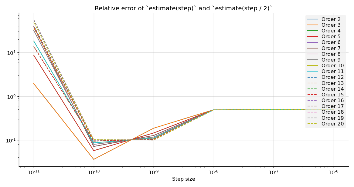
From these results I think we can possibly say that

central_fdm(3, 1, adapt=0)(df, 0, 1e-10)

gives the derivative with a relative error of at most ~5–10%. Maybe. You can extend the above experiment to find the best step size with better accuracy.

I'm thinking that just calling central_fdm(q, 1) doesn't go well because the procedure to automatically determine a step size finds one that works well for some elements of the derivative (df is multi-valued) but fails for others:

julia> (central_fdm(3, 1)(df, 0) - central_fdm(3, 1)(df, 1e-8)) ./ central_fdm(3, 1)(df, 0)
148-element Vector{Float64}:
 -1.4334788909465992e-5
  4.19189206515889e-5
  1.7207500832533594e-5
  1.720758162247681e-5
  7.056494918595109e-7
  7.682371633023401e-7
  0.010735984423210845
  0.010735984353677543
  0.005944599044609511
  0.005944599021037245
  0.016398963883520877
  0.01639896356214377
 -4.152377378291932e-5
 -4.400792286950248e-5
  4.122025356174162e-5
  4.122962192413027e-5
 -8.356807216090289e-5
  6.67547642864647e-5
  6.675479621986351e-5
  1.0483810653899413e-5
  1.0483672464959598e-5
  3.7624599200651645e-7
  3.597428654570998e-7
 -2.3663300431130233e-9
 -1.4505077031791408e-8
  ⋮
 -5.1859371908231306e-8
 -4.1797550211563575e-8
  4.2357701426808593e-7
  2.513691130573262e-7
  1.8318761071411643e-7
 -2.8739623963281802e-9
  0.002688363928732466
  0.002688364042537789
 -1.2049749539114263e-6
  0.001469467549865613
  0.0014694675608115221
  6.919078855483783e-6
  6.91907218090512e-6
 -1.7728215864604077e-7
  0.03384961097002314
  0.03384961115382243
  0.02345264321077442
  0.02345264330738625
  1.0768199313377127e-6
  1.0767593229996247e-6
  4.533637943871176e-7
  4.5046856739853824e-7
  0.0802908770638142
  0.08029087690465797
 -3.994830494965322e-6

From this it looks like the estimate works well for elements 1 to 6, but fails e.g. at the 7th. This also shows here:

julia> central_fdm(3, 1)(x -> df(x)[7], 0)
381973.2416938875

julia> central_fdm(5, 1)(x -> df(x)[7], 0)
2545.0107083557023

Two completely different answers. However, now compare

julia> central_fdm(3, 1)(x -> df(x)[7], 0, 1e-9)
416261.4394758179

julia> central_fdm(3, 1)(x -> df(x)[7], 0, 0.5e-9)
416270.4106676074

julia> central_fdm(5, 1)(x -> df(x)[7], 0, 1e-9)
416276.7878588269

julia> central_fdm(5, 1)(x -> df(x)[7], 0, 0.5e-9)
416273.4010644264

which all look very similar! I think we can conclude that the determination of the step size fails here. And the reason for this, I think, is that at the very beginning of the step size procedure, it chooses a default step size which is too large. We can (sort of) fix this by setting max_range=1e-7, which kind of prevents the step size from being much larger than order 1e-9ish:

julia> central_fdm(3, 1, max_range=1e-7)(x -> df(x)[7], 0)
416217.43166217837

julia> central_fdm(5, 1, max_range=1e-7)(x -> df(x)[7], 0)
416289.2128946737

julia> central_fdm(10, 1, max_range=1e-7)(x -> df(x)[7], 0)
416280.2540261937

And now for the whole derivative:

julia> central_fdm(10, 1, max_range=1e-7)(df, 0)
148-element Vector{Float64}:
       0.05454670451807623
      -0.027148598288693086
   14927.057274862253
  -14927.047748153713
      54.56887273995019
     -54.546313241034895
  416278.2298787704
 -416278.23286688176
       2.5523083553546857e7
      -2.552308356486684e7
  671274.6657252071
 -671274.6785747902
       0.02807019678057646
       0.020856330257093735
   19134.20051677652
  -19132.64030938499
      -1.570973683297297
   37145.68973011968
  -37145.698490679046
   12866.57077194119
  -12866.566537586232
     131.3512936174559
    -131.31100440007447
       5.693078042210595
      -5.65363796828887
       ⋮
     103.8471606229204
    -103.86459279665155
       0.06727649172635625
      66.34951781544139
     -66.38988965296109
      -0.11228568365274279
  240423.27082720457
 -240423.26070539176
      -0.014211765907845288
       5.6352528503405556e7
      -5.635252848006791e7
   11797.193874745062
  -11797.189899861567
      -0.026747502409681958
       1.0142252038092563e7
      -1.0142252022824168e7
       1.2026662874248665e7
      -1.2026662863188127e7
    1880.4665790017198
   -1880.483115881209
      14.856149949766118
     -14.883831603066223
       3.4196170336767444e6
      -3.4196170373332505e6
      -0.01321809613942529

julia> maximum((central_fdm(10, 1, max_range=1e-8)(df, 0) .- central_fdm(11, 1, max_range=1e-8)(df, 0)) ./ central_fdm(10, 1, max_range=1e-8)(df, 0))
0.07342207122310172

A better solution is probably to use a scaled version of df:

julia> maximum((central_fdm(5, 1)(x -> df(1e-6 * x), 0) .* 1e6 - central_fdm(7, 1)(x -> df(1e-6 * x), 0) .* 1e6) ./ (central_fdm(5, 1)(x -> df(1e-6 * x), 0) .* 1e6))
0.08432044412807255

I think something like this might work for you. You can prob squeeze more out of it by optimising the order of the method and further playing with the parameters to really get the best step size.

An interesting questions is whether the procedure to determine the step size automatically can be improved to also be robust in cases like this.

[thudjx]

Thanks for your reply! I do have learned a lot from your posts here! But I am sorry that I didn't make my self clear. Physically, the result of derivative should have finite value only at its 74 or 75 components, and all other components should be close to zero.

I am still not clear why there are so many divergent value components. I thought this may be caused by numerical errors. Thus I tried to use Complex{BigFloat} to store all the elements of the matrix but found that julia doesn't support this data type till now. (c.f.).

I have tried to use factor=1e10 to construct the fdm, and the result seemed much reasonable in that there are no divergent components. But I couldn't understand what is really going on here, let alone chosing a rational value for factor. Thus I tried reading the source code of FiniteDifferences, but math behind the codes is quite beyond my scope.

So the last hope for me now is to detect where the numerical divergence comes from(the effeciency of factor does imply something) and use some reasonable factor to calculate the derivative.

But before that, I have to understand how the factor works. In the source code, I find it only effects the calculation of step and accuracy. As for the related parameters, like f_error, f_error_mult is neither unclear to me. So would you please give me some more detailed explaination on that, or maybe some references? I can't appreciate more for that!

[wesselb]

Physically, the result of derivative should have finite value only at its 74 or 75 components, and all other components should be close to zero.

Ah, it seems that I converged onto a very wrong local optimum in my investigation above. 😅

I thought this may be caused by numerical errors.

Numerical errors can indeed really mess with the estimates of finite differences. Are you 100% sure that there is no error in the implementation of df? (That you're having difficulty estimating the derivative might hint at a subtle bug somewhere.)

If you want to use finite differences, one thing you can do is to do is to look at h -> (df(h) .- df(-h)) ./ (2 * h) for increasingly smalller h, e.g. h = 1e-2, h = 1e-3, etc. If I do this, the result doesn't look like it converges at all. Once you get this quantity to behave somewhat reasonably as a function of h, you should be in a good position to try central_fdm again.

So would you please give me some more detailed explaination on that, or maybe some references?

The package assumes that the error on function evaluations f(x) (df(x) in your case) is roughly factor * eps(f(x)). If the function evaluations are precise up to floating point precision (e.g. sin(1.0) would be), then factor = 1 is appropriate. If there is extra noise on the function evaluations, then you can increase factor to account for this. E.g., suppose that f(x) = 1.0 has noise on the order of 0.01. Then an appropriate factor is 0.01 / eps(1.0) = 4e-13. The reason why the noise is specified relative to the machine epsilon is to make the algorithm automatically adapt to different precisions.