Reproducing RH examples in Lightweaver

[wtbarnes]

This is perhaps less of an issue and more of a feature/docs request. My ignorance here is likely due to my unfamiliarity with Lightweaver, RH, and radiative transfer so I will apologize in advance 😅

I'm working through this toy example which uses RH (from the command line) + a combination of scripts to demonstrate the effect of the velocity on the shape of the absorption line profile around 656.25 nm. For simplicity, I'll focus just on the first part which leaves the velocity unmodified

Starting from the simple gallery example in the docs, my understanding is that I need to modify the H_6 atom that is passed to RadiativeSet in the following way:

h6 = H_6_atom()
h6.lines[4].quadrature.qCore = 25.0
h6.lines[4].quadrature.Nlambda = 200

(the 4 comes from the fact that I want to modify the first line in the Balmer series, j=2, i=1). However, my resulting line profile is

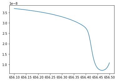
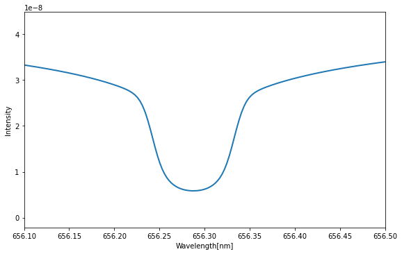
compared to the example produced in RH,

I've included the complete code to reproduce my figure below. I'm sure I'm likely doing something wrong or not completely understanding what I'm doing here!

from lightweaver.fal import Falc82
from lightweaver.rh_atoms import (H_6_atom, CaII_atom, O_atom, C_atom, Si_atom, Al_atom, Fe_atom,
                                  He_atom, Mg_atom, N_atom, Na_atom, S_atom)
import lightweaver as lw
import matplotlib.pyplot as plt
import numpy as np
import time

def synth_8542(atmos, conserve, useNe, wave):
    '''
    Synthesise a spectral line for given atmosphere with different
    conditions.

    Parameters
    ----------
    atmos : lw.Atmosphere
        The atmospheric model in which to synthesise the line.
    conserve : bool
        Whether to start from LTE electron density and conserve charge, or
        simply use from the electron density present in the atomic model.
    useNe : bool
        Whether to use the electron density present in the model as the
        starting solution, or compute the LTE electron density.
    wave : np.ndarray
        Array of wavelengths over which to resynthesise the final line
        profile for muz=1.

    Returns
    -------
    ctx : lw.Context
        The Context object that was used to compute the equilibrium
        populations.
    Iwave : np.ndarray
        The intensity at muz=1 for each wavelength in `wave`.
    '''
    # Configure the atmospheric angular quadrature
    atmos.quadrature(5)
    # Configure the set of atomic models to use.
    # Set some things specific to our example.
    h6 = H_6_atom()
    h6.lines[4].quadrature.qCore = 25.0
    h6.lines[4].quadrature.Nlambda = 200
    aSet = lw.RadiativeSet([
        h6,
        C_atom(),
        O_atom(),
        Si_atom(),
        Al_atom(),
        CaII_atom(),
        Fe_atom(),
        He_atom(),
        Mg_atom(),
        N_atom(),
        Na_atom(),
        S_atom(),
    ])
    # Set H and Ca to "active" i.e. NLTE, everything else participates as an
    # LTE background.
    aSet.set_active('H', 'Ca')
    # Compute the necessary wavelength dependent information (SpectrumConfiguration).
    spect = aSet.compute_wavelength_grid()

    # Either compute the equilibrium populations at the fixed electron density
    # provided in the model, or iterate an LTE electron density and compute the
    # corresponding equilibrium populations (SpeciesStateTable).
    if useNe:
        eqPops = aSet.compute_eq_pops(atmos)
    else:
        eqPops = aSet.iterate_lte_ne_eq_pops(atmos)

    # Configure the Context which holds the state of the simulation for the
    # backend, and provides the python interface to the backend.
    # Feel free to increase Nthreads to increase the number of threads the
    # program will use.
    ctx = lw.Context(atmos, spect, eqPops, conserveCharge=conserve, Nthreads=1)
    start = time.time()
    # Iterate the Context to convergence
    iterate_ctx(ctx)
    end = time.time()
    print('%.2f s' % (end - start))
    # Update the background populations based on the converged solution and
    # compute the final intensity for mu=1 on the provided wavelength grid.
    eqPops.update_lte_atoms_Hmin_pops(atmos)
    Iwave = ctx.compute_rays(wave, [atmos.muz[-1]], stokes=False)
    return ctx, Iwave


def iterate_ctx(ctx, Nscatter=3, NmaxIter=500):
    '''
    Iterate a Context to convergence.
    '''
    for i in range(NmaxIter):
        # Compute the formal solution
        dJ = ctx.formal_sol_gamma_matrices()
        # Just update J for Nscatter iterations
        if i < Nscatter:
            continue
        # Update the active populations under statistical equilibrium,
        # conserving charge if this option was set on the Context.
        delta = ctx.stat_equil()

        # If we are converged in both relative change of J and populations,
        # then print a message and return
        # N.B. as this is just a simple case, there is no checking for failure
        # to converge within the NmaxIter. This could be achieved simpy with an
        # else block after this for.
        if dJ < 3e-3 and delta < 1e-3:
            print('%d iterations' % i)
            print('-'*80)
            return


atmos_rest = Falc82()
wave = np.linspace(656.1, 656.5, 1000)
ctx, Iwave_rest = synth_8542(atmos_rest, conserve=False, useNe=False, wave=wave)
plt.plot(wave, Iwave_rest)

[Goobley]

Aha, good question, and something that should almost certainly be treated better in the docs.

By default, and in the way most people use it, VACUUM_TO_AIR in keyword.dat is set to TRUE for RH. Lightweaver, on the other hand, doesn't touch the output wavelength grid unless you explicitly do conversions using lw.vac_to_air. Thus, to get a +/- 0.2 nm grid around the Halpha core, you can get the line core as follows:

In [1]: from lightweaver.rh_atoms import H_6_atom

In [2]: h = H_6_atom()

In [3]: h.lines[4].lambda0
Out[3]: 656.4691622298104 
# Thus showing why the core is where it is on your plot

and then something like

halphaCore = h.lines[4].lambda0
wave = np.linspace(halphaCore - 0.2, halphaCore + 0.2, 1000)

Then if you want to plot using air wavelengths, like Ivan does, you can just call lw.vac_to_air(wave) to use as your abscissa.

Whilst it's nice to see that things work, with the way you're recomputing the spectrum using your own choice of wavelength grid (the wave variable), there's no need to adjust the quadrature on the model atom. For most things (definitely in quiet sun cases) the basic quadrature that's defined on the atom should be sufficient for the RT operator to converge, and then wave allows you to synthesise in as little, or as much detail as you want, to get a nice smooth output. Now, for very high Doppler shifts you may need to adjust the quadrature, in the way you've done here to avoid undersampling the core if it flies off into the distance. So, it is worth being aware of.

I'd definitely like to improve the docs further, currently it's essentially API documentation, but I expect it's very dense for anyone less familiar with the core materials to get into. Cheers!

[wtbarnes]

Ahh I see. Thanks! That seems to work. And thanks for the tip regarding the quadrature changes. I was not exactly sure why those were needed and was admittedly blindly trying to reproduce the RH examples.

[wtbarnes]

I'll go ahead and close this. Do you think the toy example involving the effect of velocity on the absorption profile (as shown in Ivan's notebook) would be a useful gallery example?

[Goobley]

If you would like to write up this example into a documented gallery example, I would be more than happy to accept a PR!