Spectral-preprocessing-algorithm

Common preprocessing such as sg, msc, SNV, first-order derivative, second-order derivative, etc. 近红外光谱分析技术属于交叉领域，需要化学、计算机科学、生物科学等多领域的合作。为此，在（北邮邮电大学杨辉华老师团队）指导下，近期准备开源传统的PLS，SVM，ANN，RF等经典算和SG，MSC，一阶导，二阶导等预处理以及GA等波长选择算法以及CNN、AE等最新深度学习算法，以帮助其他专业的更容易建立具有良好预测能力和鲁棒性的近红外光谱模型。 代码仅供学术使用

python版本的预处理实例

1.搭建python环境

推荐基于anaconda安装python，参考安装如下： 基于anaconda安装python

2.引入库

import numpy as np
import matplotlib.pyplot as plt
from scipy import signal
from sklearn.linear_model import LinearRegression
from sklearn.preprocessing import MinMaxScaler, StandardScaler

3.读入数据、预处理以及展示

#载入数据
data_path = './/data//data.csv' #数据
xcol_path = './/data//xcol.csv' #波长
data = np.loadtxt(open(data_path, 'rb'), dtype=np.float64, delimiter=',', skiprows=0)
xcol = np.loadtxt(open(xcol_path, 'rb'), dtype=np.float64, delimiter=',', skiprows=0)

# 绘制MSC预处理后图片
plt.figure(500)
x_col = xcol  #数组逆序
y_col = np.transpose(data)
plt.plot(x_col, y_col)
plt.xlabel("Wavenumber(nm)")
plt.ylabel("Absorbance")
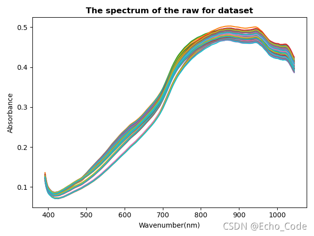
plt.title("The spectrum of the raw for dataset",fontweight= "semibold",fontsize='large') #记得改名字MSC
plt.show()

#数据预处理、可视化和保存
datareprocessing_path = './/data//dataMSC.csv' #波长
Data_Msc = MSC(data) #改这里的函数名就可以得到不同的预处理

# 绘制MSC预处理后图片
plt.figure(500)
x_col = xcol  #数组逆序
y_col = np.transpose(Data_Msc)
plt.plot(x_col, y_col)
plt.xlabel("Wavenumber(nm)")
plt.ylabel("Absorbance")
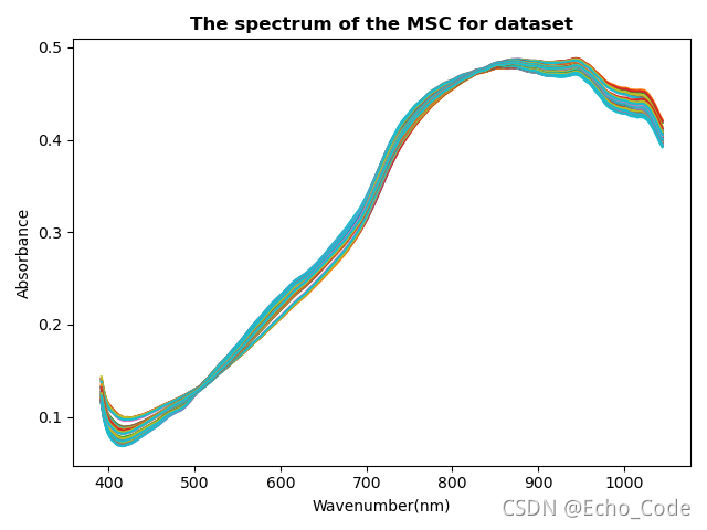
plt.title("The spectrum of the MSC for dataset",fontweight= "semibold",fontsize='large') #记得改名字MSC
plt.show()

#保存预处理后的数据
np.savetxt(datareprocessing_path, Data_Msc, delimiter=',')

4.结果(以msc为例)

原始光谱 msc预处理后 #matlab预处理的实例

matlab版本的预处理实例

1.安装matlab

受matlab版权保护，matlab安装教程自行查找

2.读入数据、预处理以及展示

clc;
clear;
% close all;
%%  打开文件
%%%%%%%%%
CA1 = csvread('D:\ProgramData\Inception\A1.csv');
Data = CA1;
%%%%%%%%%

 %% 作图，原始图
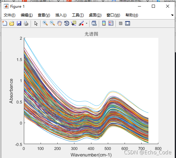
figure(1);
title('光谱图');
xlabel('Wavenumber(cm-1)');
ylabel('Absorbance');
hold on;
plot(Data');

%% 数据处理

Absorbance = Data;
[Absorbance_m,Absorbance_n]=size(Absorbance);
Absorbance_mean = mean(Absorbance);
% %% 吸光度波数
% Absorbance=data; %得到吸光度
% % Absorbance=Absorbance;
% [Absorbance_m,Absorbance_n]=size(Absorbance);
% Wavenumber=data(:,1:2:end); %得到波数
% % Wavenumber=1:141;
% Absorbance_mean=mean(Absorbance);%每个样本吸光度平均

% %% 多元散射校正MSC
% Absorbance_msc=msc(Absorbance,Absorbance_mean);
% figure(2);
% plot(Wavenumber,Absorbance_msc);
% %set(gca,'XDir','reverse'); % 横坐标从大到小
% title('多元散射校正MSC');
% xlabel('Wavenumber(cm-1)');
% ylabel('Absorbance');
%% 多元散射校正MSC
msc_file_name =  'D:\DsekTop\MSCA1.csv';
Absorbance_msc=msc(Absorbance,Absorbance_mean);
csvwrite(msc_file_name,Absorbance_msc,0,0);
figure(2);
title('多元散射校正MSC');
xlabel('Wavenumber(cm-1)');
ylabel('Absorbance');
hold on;
plot(Absorbance_msc');

3.结果(以msc为例)

原始光谱

MSC预处理后光谱