[Question] Candidate sampling probability for Mixed Negative Sampling

[OmarMAmin]

Hi Team,

Sorry for posting many questions, I hope this will help others navigate through building high quality models :)

I've trained a two tower model, and checking the possibility of using it directly, but from inspecting a few outputs I guess part of the retrieval is focused on popular items even if it's not that relevant to the user context (previous searches, previous items, previous purchases, time of the day .. etc), I'm not sure if i need to add more features, tune it further .. etc (will do so anyway).

But I guess using Mixed Negative Sampling would help with that, as its main target is to make the model better understand how to distinguish between frequent items and non-frequent items --> so it'll be a bit more confident in ranking non-popular items higher when it see the context to, but I'm wondering how to calculate the candidate sampling probability, for the two tower model, i calculated it using the item frequency in training set (# appearences/ # all interactions)

Quoting from the paper, it seems that the way we should be calculating the candidate_sampling_probability should be different as the We're sampling the other batch uniformly, but how it should be different? My guess that it would be a weighted average of

sampling_probability = (batch_1 * item_frequency_in_training + batch_2 * uniform_frequency) / (batch_1 + batch_2) batch_1: the original batch size for two tower model batch_2: the complementary random negative batch size

Can you please confirm my understanding for MNS impact (retrieving more high quality results)? and the way to calculate the sampling_probability?

Thanks :)

[patrickorlando]

Your calculation is correct @OmarMAmin.

[hkristof03]

In the implementation, the global negatives are sampled uniformly from the item corpus. I understand that in the original training dataset each sampling probability is adjusted based on the above equation:

# batch_1: the original batch size for two tower model
# batch_2: the complementary random negative batch size

sampling_probability = (batch_1 * item_frequency_in_training + batch_2 * uniform_frequency) / (batch_1 + batch_2)

But for the Retrieval task, the additional sampling probabilities corresponding to the global negatives should be appended. I think if I have an item corpus with cardinality of 20_000, then the corresponding sampling probabilities for the global negatives are [1 / 20_000, ..., 1 / 20_000], right?

[patrickorlando]

@hkristof03 you are correct, but regardless of the position in the row, the softmax is calculated over all negatives. The sampling probability for an item should be overall the probability that it is sampled as an item in the batch. This is irrespective of which sampling method it came from. There is only one value for this probability per item, which is why the equation above is used.

For example, for an item with a very low frequency, adding uniform negatives will make it much more likely to be sampled as a negative in any given batch (and therefore appearing in the denominator of the softmax for any given example).

[OmarMAmin]

@patrickorlando I got back to the paper and the section about estimating sampling probability

In this section, we elaborate the streaming frequency estimation used in Algorithm 1. Consider a stream of random batches, where each batch contains a set of items. The problem is to estimate the probability of hitting each item y in a batch. A critical design criterion is to have a fully distributed estimation to support distributed training when there are multiple training jobs (i.e., workers). In either single-machine or distributed training, a unique global step, which represents the number of data batches consumed by the trainer, is associated with each sampled batch. In a distributed setting, the global step is typically synchronized among multiple workers through parameter servers. We can leverage the global step and convert the estimation of frequency p of an item to the estimation of δ, which denotes the average number of steps between two consecutive hits of the item. For example, if one item gets sampled every 50 steps, then we have p = 0.02. The use of global step offer us two advantages: 1) Multiple workers are implicitly synchronized in frequency estimation via reading and modifying the global step; 2) Estimating δ can be achieved by a simple moving average update, which is adaptive to distribution change

I guess this means that the candidate sampling probability should be calculated as the probability of getting sampled in a batch, so it should be prob_item = itemcount/datasetsize sampling_prob = 1 - (1 - prob_item) ** batchsize

I saw it in multiple issues, calculated as the item frequency which represent the sampling probability if batch size is only 1 right? but if we are sampling 1024 different interactions, the probability of being sampled in a batch would be > item frequency right?

[hkristof03]

@patrickorlando to clarify it totally, am I right that the sampling probabilities should be computed from the train dataset for each item ID, then these probabilities should be joined to the validation dataset and the item dataset (for mixed negative sampling)? Thanks in advance!

[OmarMAmin]

For Mixed Negative Sampling i guess the sampling probability should be mns_sampling_prob = 1 - (1 - uniform_prob) * (1 - sampling_prob) sampling_prob is the prob of getting sampled from the training dataset (once or in a batch of size N) uniform_prob is the prob of getting sampled uniformly as a negative sample from the MNS batch (once or in a batch of size M)

I revisited the formula that i included in the issue as in my case I've some popular items that almost appear in every batch, so regardless if we're doing mixed negative sampling or not it'll be definitely there in each batch, so it'll be a negative for all other pairs, so no need for correction here, even if the other negative batch has sampling of 0.01 probability, the item is already there in the other batch.

So it can't be a weighted average as if so, the prob will be less than 1 which doesn't make sense if the item is sampled in the first batch independently of the way of the second batch, so the overall probability for the popular item should increase not be somewhere between the two probabilities.

[patrickorlando]

sampling probabilities should be computed from the train dataset for each item ID, then these probabilities should be joined to the validation dataset and the item dataset (for mixed negative sampling)?

Yes, that's my understanding @hkristof03. However, during validation, when the FactorizedTopK metric is calculated over the whole item corpus, sampling isn't used, and TFRS won't make use of these sampling probs. I think they are used however for any batch metrics, (because the classes are sampled).

[patrickorlando]

@OmarMAmin I can't find the section you quoted in that paper, and I don't quite follow your calculation. I'll walk you through my understanding.

Firstly, the section is describing how to estimate the item frequency, not the probability of an item being sampled. Let's clarify this part first. If we are estimating the frequency, without mixed negative sampling, then it would be

freq_i = (item_count_i/dataset_size) * batch_size
       =  Q_i * batch_size

If an item appears once every 50 batches, it will have frequency 0.02, if the batch size is 1024, then it's streaming sampling probability is 0.02/1024 = 1.9E-5.

Let's go with the frequency estimation as our logit correction.

Now if we use one of the laws of logarithms, log(a*b) = log(a) + log(b), so our sampling corrected logits y'_i would be

y'_i = y_i - log(Q_i*batch_size)
     = y_i - log(Q_i) - log(batch_size)

Importantly, the last term is applied to every logit and it doesn't depend on y. It therefore becomes a constant factor that simply shifts the logits, but will have zero effect on learning. We can prove the probabilities coming out of the softmax will be identical.

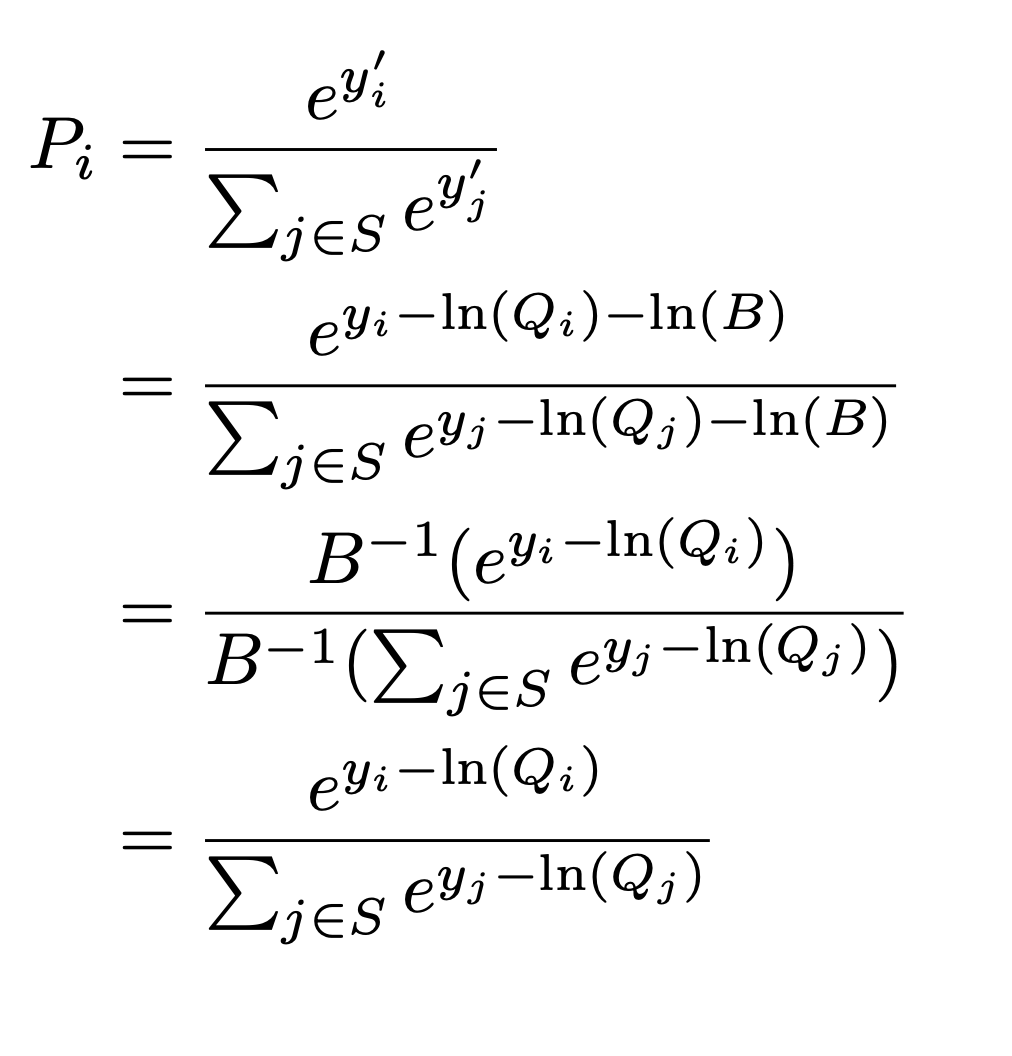
Where S is the set of sampled items in the batch and B is the batch size.

So essentially, using the frequency or the sampling probability is the same, but amounts to shifting the logits by a constant factor which depends only on the batch size.

Now, assuming we go with the frequency estimation route and we want to calculate it for MNS. In this case the expected frequency for an item would be

freq_i  = dataset_prob_i*batch_size + uniform_prob_i*uniform_batch_size

that is how often we expect to see an item in a given batch. Now again, we could scale this by any constant factor, and one natural reason to do so is to describe this as simply the probability of an item occupying a spot in the batch, which would be

Q_i  = (dataset_prob_i*batch_size + uniform_prob_i*uniform_batch_size) / (batch_size + uniform_batch_size)

Essentially we can use item frequency, or item sampling probability, or any factor of it. However I don't quite understand how you arrived at sampling_prob = 1 - (1 - prob_item) ** batchsize.

[OmarMAmin]

Thanks @patrickorlando for your reply.

I was referring to the original paper, section 4

From what i understand

1. They defined the sampling probability as the inverse of the number of steps between seeing a sample in a batch (as quoted from the paper, For example, if one item gets sampled every 50 steps, then we have p = 0.02).
2. We're applying the logit correction as some negatives are sampled more than other due to the in batch negatives

Case1: we're not using mixed negative sampling Assume that an item is extremely popular it appears in 50% of the interactions.

Probability of sampling this item in a batch of 1 would be 0.5, in a batch of 2 would be 1 - (0.5)*(0.5), which represent probability of being sampled in either the first item in the batch or the second item, for a batch of 1024, you'll definitely see this item in every batch, so no logit correction needs to be applied there (please correct me if i'm wrong)

Case2: we're now using mixed negative sampling Same popular item, with probability ~= 1 of being sampled in every single batch, adding another batch of negatives doesn't change the fact that this popular item will almost always be there, doing the weighted average assumes that we're merging the two populations (uniform negatives, in-batch negatives), and then we're sampling a new batch of size 1024 or 2048 from the mixed population.

From what i understand, we're sampling two independent batches from two different distributions, and then trying to estimate a single item sampling probability in both in the mixed batch, so i guess it should be probability of being in either of both batches right?

In that case I calculated it as:

p_mns = 1 - A * B
A = probability of not being in the in-batch negatives
B = probability of not being in the uniform negatives batch
A = (1 - prob_item) ** inbatch_negatives_batch_size
B = (1- uniform_prob) ** mns_batch_size

Assuming sampling is done with replacement

This is what i understood from the paper, please let me know if i got sth wrong

[patrickorlando]

Interesting @OmarMAmin, I've read the section and as far as I can tell, it does seem to estimate the frequency in the way you've described. It's not really aligned with how I understand the non-streaming case to function. This definition and proof here, defines the Log(Q) correction as:

Q(y|x) is defined as the probability (or expected count) according to the sampling algorithm of the class y in the (multi­)set of sampled classes given the context x.

And when deriving the correction term, it states:

In “Sampled Softmax”, for each training example (x_i , {t_i}) , we pick a small set S_i ⊂ L of “sampled” classes according to a chosen sampling function Q(y|x) . Each class y ∈ L is included in S independently with probability Q(y|x_i)

The streaming calculation in the paper you linked doesn't align with this. It truncates the frequency. If one item appears on average four times in a single batch, and another appears on average once in a batch, then their correction term will be the same. This would appear to introduce bias into the learned relative log probabilities. For example if you take the limit as the batch size approaches the entire training set size, then effectively no correction is applied, despite the varying number of each class being used as a negative.

[OmarMAmin]

Thanks for the reply, tbh I didn't fully get the logit correction yet, but when i got back to the papers that discussed that at first, I guess the distinction here, is that each sampled item is a shared negative for the whole batch, as if it was randomly sampled as negative for each row in the batch, unlike the regular sampled softmax which is sampling negatives for each element in the batch independently, i guess that's why the calculation might differs depending on which version of sampled softmax is being used but tbh I'm not confident yet about this conclusion :D, will dig deeper into it.

[caesarjuly]

@OmarMAmin I just came across this thread and learned many things from your ideas. Thanks! I also implemented the streaming version of frequency estimation from the sampling bias correction paper. If you leverage this implementation, you can skip the manual calculation and get the frequency result on the fly. I put the code example and the usage here. This is not a perfect version for continual or incremental training, but it is a good start for offline training. For real continual training, I need to support expiration logic too. The recall diff is listed below in my mini example training on the MovieLens dataset.

	Recall@100
Without SBC	0.1236
With SBC	0.2696

I also wrote a blog talking about the details :).

[OmarMAmin]

This is really interesting results, Thanks @caesarjuly for sharing the improvement, Can I ask what is the catalogue size in your case?

[caesarjuly]

@OmarMAmin I have deployed this approach in a production environment. My case is an incremental training scenario, hourly load and fine-tune a model and then deploy this model to production. My vocabulary size is not very big, about 50k per day, and it has run smoothly for over a month. The total vocabulary size is around 1m. And the whole model size increased by <100M. You can calculate the memory consumption by hand. We have 2 hash tables, and each item will occupy one key of 8 bytes (I use string as the key, this will depend on your string length) and one value of 8 bytes. Suppose we have 1m items, the total memory footprint will be 2*16*1,000,000/1024/1024 = 30M. Regarding the model performance, I have tested it vs. a naive sampling strategy (for each positive sample, sampling N negatives as the training input). The result is almost the same. I plan to support an expiration function in the next week. I will let you know when finished. Btw, I refactored my code recently. Some links are incorrect in my previous comment. I just fixed them.

[OmarMAmin]

Thanks for sharing @caesarjuly (Y)

[caesarjuly]

@OmarMAmin I read your discussion above. I think the original two papers listed above don't discuss how to handle in-batch collisions(the same item appears several times within 1 batch) in detail. According to the algorithm, the sampling bias correction paper ignores the collision since the frequency estimation is based only on training steps. I guess this is because they have a huge corpus, and the collision probability is relatively tiny. Regarding your popular item domination issue, I have some discussion in my post.

We want a model that has a good resolution on both the popular items and long-tail items

If the sampling distribution is too close to the uniform distribution, then the popular items can easily win because of their intrinsic popularity. The retrieval results will be dominated by them

If the sampling distribution is too close to the unigram distribution, then the popular items will be down boost too much as they are frequently chosen as the negatives

So here is an internal balance requirement between these two sampling streams

In general, I think there is 2 bias need to be corrected.

1. Negative sampling bias, corrected by Log(Q) correction. This bias harms popular items. Without extra negatives and bias correction, the target logits will be P - log(Q). Since the popular items have a large log(Q), the final probability will be punished hard.
2. Selection bias, corrected by MNS. This bias harms the long-tail items. The target logits will be P without extra negatives but with bias correction. This is what we want. But as discussed in the MNS paper, there is a selection bias here. So we need to provide extra uniform samples to correct this bias.

Update: I have upgraded my sampling bias correction class to support expiration functions. Now it's completed.

[houghtonweihu]

Hi @patrickorlando I saw that you have helped many people on this topic. I am curious if you have any inside or advice to help me understand these two questions:

 How to know the Rank model improves the output of the Retrieval model in the case of MovieLens dataset? #690
 https://github.com/tensorflow/recommenders/issues/690

 How to know better evaluation metrics for Retrieval or Rank will translate into better actual recommendations in the case of MovieLens dataset? #691
 https://github.com/tensorflow/recommenders/issues/691

  Thanks for your help!