papernotes
 papernotes copied to clipboard
Adversarial Contrastive Estimation
Metadata
- Authors: Avishek Joey Bose, huan ling, Yanshuai Cao
- Organization: Borealis AI & University of Toronto
- Conference: ACL 2018
- Paper: http://aclweb.org/anthology/P18-1094
- Blog: https://www.borealisai.com/en/blog/adversarial-contrastive-estimation-harder-better-faster-stronger/
- Author's original project paper: https://joeybose.github.io//assets/active-ace.pdf (mentions background of active learning)
Summary
This paper proposes to augment the negative sampling process in contrastive learning with an adversarially learned conditional distribution, resulting in a negative sampler that adapts to the data distribution, training dynamics and finds harder negatives (refered to as Adversarial Contrastive Estimation (ACE)). They demonstrate the efficacy and generality of ACE on learning word embeddings, order embeddings and knowledge graph embeddings.
Motivation of This Paper (Problems of Previous Approach)
- Current negative sampling process does not condition on positive example (e.g., random sampling).
- Furthermore, it usually encodes a human prior as to what constitutes a hard negative example, rather than being learned from data.
- Easy negative examples are sub-optimal for learning discriminative representation as they do not force the model to find critical characteristics of observed positive examples.
- Even if hard negatives are occasionally reached, the infrequency leads to slow convergence.
Background: Contrastive Learning
Contrastive learning is a sampling-based learning method that contrasting losses on observed positive examples with those on sampled fictitious negative examples, trying to minimize loss on positive ones while maximizing it on negative ones. One of the popular algorithms is Noise Contrastive Estimation (NCE) and has been applied on learning word embeddings. See the bellowing comment for Notes on Noise Contrastive Estimation.
Why contrastive learning?
- Computational efficiency, especially when the vocabulary is large.
- Modeling need: For example, modeling entity relations in a vector space naturally leads to a distance-based score to be minimized for observed entity-relation-entity triplets.
Objective in general form:
In most general form, the objective of contrastive learning:
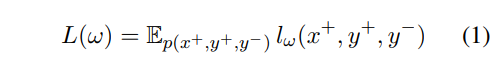
- l_ω(x+, y+, y-) is the loss that scores a positive example (x+, y+) against a negative one (x+, y-).
- E_{p(x+, y+, y-)}(.) denotes expectation w.r.t. the joint probability distribution over positive and negative examples.
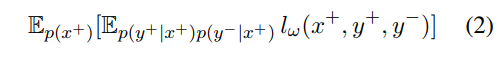
By the law of total expectation and the fact that given x+, the negative sampling y- is not dependent on the y+ (i.e., p(y+, y- | x) = p(y+ | x+) p(y- | x+)). Thus, rewrite Eq. 1 as:
Non-separable loss and separable loss
There are two cases of l_ω(x+, y+, y-) depends on different problems:
- Non-separable loss: l_ω(x+, y+, y-) = max(0, η + s_ω(x+, y+) - s_ω(x+, y-)). (Triplet ranking loss)
- Separable loss:
 then, Eq 2. becomes:
 Note that for generality, the loss function for negative samples, denoted by s˜_ω, could be slightly different from s_ω.
In NCE, we make p(y-|x+) to be some unconditional p_{nce}(y-) in Eq. 2 or 3, which leads to efficient computation but sacrifices the sampling efficiency (y- might not be a hard negative example).
Purposed Method: Adversarial Contrastive Estimation (ACE)
To remedy the above problem of a fixed unconditional negative sampler p_{nce}(y-), ACE augments it into an adversarial mixture negative sampler: λ p_{nce}(y-) + (1 − λ) gθ(y-|x+).
Training objectives for embedding model (discriminator parameterized by ω) and gθ (generator parameterized by θ)
The Eq. 2 can be written as (ignore E_p(x+) for notational brevity):

Then, learn (ω, θ) with GAN-style training:
 The generator gθ is trained via policy gradient ∇θL(θ, x):
 where the expectation is w.r.t. p(y+|x) gθ(y-|x), and the discriminator loss l_ω(x, y+, y-) acts as the reward.
Note: The generator aims to maximize L(.), thus the reward is l_ω(x, y+, y-)
Question: Many papers did not add negative sign to the reward term. Due to the update rule of REINFORCE is gradient ascent, I think there is no negative sign to the reward term.

We can also rewrite L(ω, θ; x) when l_ω is separable-loss:

The bellowing is the derivation of L(ω, θ; x) with separable-loss l_ω:

Question: The authors ignore λ terms in the Eq. 7, which 'm not sure whether it's correct or not.
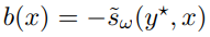
When in separable-loss case, the reward term in policy gradient ∇θL(θ, x) for updating the generator would be: −s˜(x+, y−), since only the last term depends on the generator parameter θ. (<- the original paper writes ω which is wrong!).
Note: The generator aims to maximize L(.), which is equivalent to minimize the last term -E_{gθ(y-|x)} s˜(x+, y−). Thus, the reward is −s˜(x+, y−). Again if in non-separable case, the reward term becomes l_ω(x, y+, y-).
Techniques for Further Improvement
Regularization for gθ: Entropy and training stability
To avoid gθ mode collapse in GAN training, they propose to add a regularization term for gθ to encourage it to have high entropy.
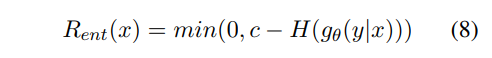 where H(gθ(y-|x)) is the entropy of gθ, and c = log(k) is the entropy of a uniform distribution over k choices. Intuitively, R_{ent} expresses the prior that the generator should spread its mass over more than k choices for each x.
H(x) = - Σ_{i}^{k} P(x_i) log P(x_i) (by entropy definition) = - k * (1/k) log (1/k) (by uniform distribution) = -log (1/k) = -log k^(-1) = log k
Note that it is actually "max" instead of "min" in Rent equation. (I just confirmed it with the authors).
Handling false negatives
ACE samples false negatives more than NCE. Thus, two strategies are further introduced (although entropy regularization reduces this problem):
- Detect if a negative sample is an actual positive observation. If so, its contribution to the loss is given a zero weight in ω learning step , and the reward for false negative samples are replace by a large penalty for gθ.
- Prevent null computation when gθ learns to sample false negatives, which are subsequently ignored by the discriminator update for ω.
Variance reduction
They subtract the baseline from reward to reduce the variance of policy gradient estimator with self-critical baseline method, where the baseline is:
- In non-separable loss case:

- In separable loss case:

Note: Make sampling better than greedy decoding.
Improving exploration in gθ by leveraging NCE samples
Reweighting the reward term in Eq. 6 by gθ(y−|x) / p_{nce}(y−).
My understanding is that, if p_{nce} has already sampled y-, then make gθ(y−|x) sample y- less. Authors state that this is essentially "off-policy" exploration in reinforcement learning since NCE samples are not drawn according to gθ.
Experiment Settings
Word embeddings
- Evaluate models trained from scratch and fine-tuned Glove
- Dataset: Rare word dataset & WordSim-353
Hypernym prediction
- Hypernym pairs are created from the WordNet hierarchy's transitive closure.
- Use released random development split and test split from Vendrov et al. (2016), which both contain 4000 edges.
Knowledge graph embeddings
- Use TransD as base model.
- Dataset: WN18
Experiment Results
 (ACE: mixture of p_{nce} and gθ; ADV: only gθ)
- Figure 2 (hypernym prediction task): Loss on the ACE negative terms collapses faster than on the NCE negatives. After adding entropy regularization and weight decay, the generator works as expected.
- Figure 3 (word embedding task): ACE converges faster than NCE after one epoch.
- Figure 4 (word embedding task): The discriminator's loss on gθ is always higher than on p_{nce}, indicating that the generator is indeed sampling harder negatives.
 .
.
- ACE embeddings have much better semantic relevance in a larger neighborhood (nearest neighbor 45-50).

- Table 2: ACE on RW is not always better and for the 100d and 300d Glove embeddings is marginally worse. However, on WordSim353 ACE does considerably better across the board to the point where 50d Glove embeddings outperform the 300d baseline Glove model.
 (Knowledge graph embedding training progress. Ent: Entropy Regularization; SC: Self-critical baseline; IW: off-policy learning)
- All variants of ACE converges to better results than NCE.
- With Ent > without Ent
- Without SC, learning could progress faster at the beginning but the final performance suffers slightly.
- The best performance is obtained without off-policy learning of the generator.
 (Knowledge graph embedding performance)
Limitations
- When the generator's softmax is large, the current implementation of ACE training is computational expensive. The computational cost can be potentially reduced via techniques which aim to tackle softmax bottleneck ("augment and reduce" variational inference , adaptive softmax, "sparsely-gated” softmax, etc.)
- Theoretical connections between GANs and maximum likelihood estimation (MLE) are still unknown. As noted in Goodfellow (ICLR 2015), GANs do not implement MLE, while NCE has MLE as an asymptotic limit. And the tools for analyzing the equilibrium of a min-max game where players are parametrized by deep neural nets are currently not available.
Reference
- Incorporating GAN for Negative Sampling in Knowledge Representation Learning by Wang et al. AAAI 2018.
- Order-embeddings of images and language by Vendrov et al. ICLR 2016.
- On Distinguishability Criteria for Estimating Generative Models by Ian J. Goodfellow. ICLR 2015.
- Notes on Noise Contrastive Estimation and Negative Sampling by Chris Dyer.
- On word embeddings - Part 2: Approximating the Softmax by Sebastian Ruder.
Notes on Noise Contrastive Estimation (NCE)
Idea
In neural language modeling, computing the probability normalization term in softmax is expensive. Thus, NCE and its simplified variants, negative sampling transform the computationally expensive learning problem into a binary classification proxy problem that use the same parameters θ to distinguish samples from the empirical distribution (i.e., (w+, c)~p*(w|c)) from samples generated the noise distribution q(w) (i.e., (w-, c)~q(w)). In practice, q(w) is a uniform unigram distribution). Note: we denote w+ is a positive example, w- is a negative example and c is a given condition (context).
Neural language modeling: Train a neural network pθ(w | c) = uθ(w, c) / Z(c) to approximate the empirical (training data) distribution p*(w|c) as closely as possible. uθ(w, c) = exp sθ(w, c), where sθ(w, c) is a differentiable function that assigns score to a word in context. Z(c) is the probability normalization term.
Training
During training, we form the training data by sampling one positive example (w+, c) and k negative examples (w-, c) with labels 1 and 0 respectively.
Formulate the above description into a mathematical expression:

And using the definition of conditional probability:

NCE replaces the empirical distribution p*(w|c) with the model distribution pθ(w|c) and makes 2 assumptions to solve the computation problem in Z(c):
- For every c, use a parameter z_c to estimate Z(c).
- For neural networks with lots of parameters, it turns out that fixing z_c = 1 for all c is effective. This assumption reduces z_c and encourages the model to have "self-normalized* outputs (i.e., Z(c) ≈ 1).
Making these assumptions, rewrite the p*(w|c) (which is replaced with pθ(w|c)) to uθ(w, c) in the above equations:

Note: In simplified variant of NCE, negative sampling, the term k × q(w) becomes to 1. It is equivalent to NCE when k = |V| and q is uniform.
The objective function of maximizing the above conditional log-likelihood of D in above equations would be:

Since the expectation of the second term is still a difficult summation, we use Monte Carlo sampling to approximate the expectation term:

Asymptotic Analysis

Read More
- Conditional Noise-Contrastive Estimation of Unnormalised Models [pdf] [supp] by C. Ceylan, and M. Gutmann. ICML 2018.
- Learning word embeddings efficiently with noise-contrastive estimation [pdf] [poster] by Andriy Mnih and Koray Kavukcuoglu. NIPS 2013.
- A fast and simple algorithm for training neural probabilistic language models [pdf] [slides] [poster] by Andriy Mnih and Yee Whye Teh. ICML 2012.
- Noise-contrastive estimation: A new estimation principle for unnormalized statistical models [pdf] [slides] by M. Gutmann, and A. Hyvärinen. AISTATS 2010.