effectsize
 effectsize copied to clipboard
new effect size: `semipartialR2`
First attempt at providing the sr2 (#154). There are currently three aliases. Demo:
devtools::load_all(".")
library(rempsyc)
m <- lm(mpg ~ cyl + disp + hp * drat, data = mtcars)
semipartialR2(m)
#>     Parameter         sr2
#> 1 (Intercept)          NA
#> 2         cyl 0.007338114
#> 3        disp 0.018414581
#> 4          hp 0.005330776
#> 5        drat 0.023587381
#> 6     hp:drat 0.010561014
deltaR2(m)
#>     Parameter         sr2
#> 1 (Intercept)          NA
#> 2         cyl 0.007338114
#> 3        disp 0.018414581
#> 4          hp 0.005330776
#> 5        drat 0.023587381
#> 6     hp:drat 0.010561014
sr2(m)
#>     Parameter         sr2
#> 1 (Intercept)          NA
#> 2         cyl 0.007338114
#> 3        disp 0.018414581
#> 4          hp 0.005330776
#> 5        drat 0.023587381
#> 6     hp:drat 0.010561014
We can setup a full dataframe to compare with rempsyc::nice_lm
data.frame(
  `Dependent Variable` = insight::find_response(m),
  Predictor = sr2(m)$Parameter,
  df = insight::get_df(m),
  b = insight::get_parameters(m)$Estimate,
  t = insight::get_statistic(m)$Statistic,
  p = parameters::p_value(m)$p,
  sr2 = sr2(m)$sr2
)
#>   Dependent.Variable   Predictor df           b          t          p
#> 1                mpg (Intercept) 26 14.13406373  1.2111203 0.23674315
#> 2                mpg         cyl 26 -0.80528708 -0.9602187 0.34579043
#> 3                mpg        disp 26 -0.01695619 -1.5211039 0.14030351
#> 4                mpg          hp 26  0.06152000  0.8184142 0.42055869
#> 5                mpg        drat 26  4.76308511  1.7215427 0.09703178
#> 6                mpg     hp:drat 26 -0.02209297 -1.1519424 0.25982735
#>           sr2
#> 1          NA
#> 2 0.007338114
#> 3 0.018414581
#> 4 0.005330776
#> 5 0.023587381
#> 6 0.010561014

nice_lm(m)
#>   Dependent Variable Predictor df           b          t          p         sr2
#> 1                mpg       cyl 26 -0.80528708 -0.9602187 0.34579043 0.007338114
#> 2                mpg      disp 26 -0.01695619 -1.5211039 0.14030351 0.018414581
#> 3                mpg        hp 26  0.06152000  0.8184142 0.42055869 0.005330776
#> 4                mpg      drat 26  4.76308511  1.7215427 0.09703178 0.023587381
#> 5                mpg   hp:drat 26 -0.02209297 -1.1519424 0.25982735 0.010561014
Same result, yeah! :)
Created on 2022-10-02 with reprex v2.0.2</sup](https://reprex.tidyverse.org%29%3C/sup)>
I'm currently inclined to have a simplified function for lm models only, using the model's matrix (instead of formula interface), which will allow for interaction support.
The docs can point to the dominance analysis function in parameters for other model types and more verbose info / options.
There's a paper for parametrically computing CIs too (~need to find it again~ https://sci-hub.se/10.1177/0013164410379335).
Wdyt?
I'm currently inclined to have a simplified function for lm models only, using the model's matrix (instead of formula interface), which will allow for interaction support.
The current version does support interactions (as shown in the reprex) and takes the model object directly. It is also a simplified version that supports lm models only for now. Does that address your first point? And what do you mean using the model's matrix (instead of formula interface)? Is that what I am already doing or not?
The docs can point to the dominance analysis function in parameters for other model types and more verbose info / options.
Good idea, I can add that.
There's a paper for parametrically computing CIs too (need to find it again https://sci-hub.se/10.1177/0013164410379335).
Cool, thanks, will have a look and see if I can extract the formula to code it!
Codecov Report
Merging #511 (1617863) into main (ea251c7) will increase coverage by
0.13%. The diff coverage is98.27%.
@@            Coverage Diff             @@
##             main     #511      +/-   ##
==========================================
+ Coverage   90.52%   90.66%   +0.13%
==========================================
  Files          54       55       +1
  Lines        3177     3235      +58
==========================================
+ Hits         2876     2933      +57
- Misses        301      302       +1
| Impacted Files | Coverage Δ | |
|---|---|---|
| R/convert_stat_to_anova.R | 88.05% <ø> (ø) |
|
| R/convert_stat_to_r.R | 95.12% <ø> (ø) |
|
| R/effectsize.R | 96.77% <ø> (ø) |
|
| R/equivalence_test.R | 80.55% <ø> (ø) |
|
| R/eta_squared-main.R | 93.94% <ø> (ø) |
|
| R/interpret_cfa_fit.R | 100.00% <ø> (ø) |
|
| R/r2_semipartial.R | 98.27% <98.27%> (ø) |
Help us with your feedback. Take ten seconds to tell us how you rate us. Have a feature suggestion? Share it here.
Ok I added documentation pointing to the dominance analysis function in parameters for other model types and more verbose info / options. However, I'm afraid people checking the dominance analysis documentation will be confused, as again there is no mention of sr2, or what/where to look in the output, etc.
However, I'm afraid people checking the dominance analysis documentation will be confused, as again there is no mention of sr2, or what/where to look in the output, etc.
I agree. Perhaps a separate issue about that can be raised in parameters?
Also, a suggestion for a slightly different method that can deal with interactions (and gives CIs maybe?)
Code
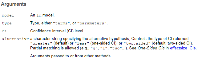
semipartial_r2 <- function(model, type = c("terms", "parameters"),
                          ci = 0.95, alternative = "greater",
                          ...) {
  UseMethod("semipartial_r2")
}

semipartial_r2.lm <- function(model, type = c("terms", "parameters"),
                           ci = 0.95, alternative = "greater",
                           ...) {
  type <- match.arg(type)

  mf <- stats::model.frame(model)
  mm <- stats::model.matrix(model)
  mterms <- stats::terms(model)

  y <- mf[[1]]

  if (type == "terms") {
    out <- data.frame(Term = attr(mterms,"term.labels"))
    idx <- attr(mm, "assign")
    idx_sub <- idx[idx > 0]
  } else {
    out <- data.frame(Parameter = colnames(mm))
    out <- subset(out, Parameter != "(Intercept)")
    idx <- seq.int(ncol(mm))
    idx_sub <- idx[colnames(mm)!="(Intercept)"]
  }

  tot_mod <- if (attr(mterms,"intercept") == 1) {
    stats::lm(y ~ 1 + mm)
  } else {
    stats::lm(y ~ 0 + mm)
  }

  sub_mods <- lapply(unique(idx_sub), function(.i) {
    if (attr(mterms,"intercept") == 1) {
      stats::lm(y ~ 1 + mm[,.i!=idx])
    } else {
      stats::lm(y ~ 0 + mm[,.i!=idx])
    }
  })

  tot_r2 <- performance::r2(model)[[1]]
  sub_r2 <- lapply(sub_mods, performance::r2)
  sub_r2 <- sapply(sub_r2, "[[", 1)

  out$semipartial_r2 <- unname(tot_r2 - sub_r2)

  if (!is.null(ci)) {
    tot_df_model <- insight::get_df(model, type = "model")
    sub_df_model <- tot_df_model - sapply(sub_mods, insight::get_df, type = "model")
    df_res <- stats::df.residual(model)

    F_stat <- (out$semipartial_r2 / (1 - out$semipartial_r2)) * (df_res / sub_df_model)

    out <- cbind(out, effectsize::F_to_eta2(F_stat, sub_df_model, df_res, ci = ci, alternative = alternative)[,2:4])
  }

  out
}
mod <- lm(log(mpg) ~ factor(cyl) + am * hp, mtcars)

semipartial_r2(mod)
#>          Term semipartial_r2   CI CI_low CI_high
#> 1 factor(cyl)    0.024978297 0.95      0       1
#> 2          am    0.002787493 0.95      0       1
#> 3          hp    0.045765510 0.95      0       1
#> 4       am:hp    0.005961929 0.95      0       1
Created on 2022-10-16 by the reprex package (v2.0.1)
Also, a suggestion for a slightly different method that can deal with interactions
I know you've mentioned this before, but I don't understand this point. Again, my current code and original reprex can already deal with interactions, can it not? E.g., just the relevant lines about the interaction between hp and drat:
m <- lm(mpg ~ cyl + disp + hp * drat, data = mtcars)
semipartialR2(m)
#>     Parameter         sr2
#> 6     hp:drat 0.010561014
(and gives CIs maybe?)
That's cool. Why the maybe though? Is it because you're not sure whether the CI properties are valid when converting from sr2 to F to eta2? Or is it simply the CI of eta2 instead of the sr2 (I know the two are very close, but still)?
I've tried your function on my original reprex example see if it gives the same result. My first observation is that the 95% CI lower and upper bounds are still 0 and 1 even when not using the dichotomous am variable. But even with am, it should not have been binary like this since the sr2s are continuous, no?
Beside that problem, our two methods have identical sr2 values.
(Also sapply is not recommended but of course that's minor as we can change it easily.)
However, I'm afraid people checking the dominance analysis documentation will be confused, as again there is no mention of sr2, or what/where to look in the output, etc.
I agree. Perhaps a separate issue about that can be raised in parameters?
I'm not entirely convinced that improving parameters::dominance_analysis documentation is the way to go (though perhaps it is). The reason is that the dominance analysis output provides a bunch of information for people looking to do dominance analysis. People looking simply for the sr2 for simple regression that report it like they report R2 will not look there IMO.
One could argue, but we could mention the sr2 in the dominance analysis documentation just in case. We could. But then would we not have to add descriptions for alternative names for every single value of the output? It would feel a bit arbitrary to me to just do it for one and not the others. And then it could be a lot of information.
Linking to parameters::dominance_analysis from effectsize::semipartialR2 does make sense to me though.
Finally, I've looked at Algina, Keselman, & Penfield (2010) again but don't really understand how to convert their formulas to an R function to compute the parametric CI. My math competencies are very basic 😬
Just some thoughts; currently the 3 aliases are
semipartialR2, deltaR2, sr2
My thoughts are that I'd drop the last short form (we tend to favor explicit forms). And I would also stick with only one version semipartial or delta (and then put in the documentation title for e.g., "Semi-partial R2 (aka delta R2)"), whichever makes more "sense"
also, we use r2() and e.g., r2_nakagawa() (albeit in performance), so should we instead use something like r2_semipartial()? Especially since we don't use a lot of camelCase?
Also pretty printing (in parameters?) with something like R2 (semi-partial) instead of sr2?
I like r2_semipartial best, I think.
If this will be in the effectsize package, it will have the effectsize_table class, and a nice printing method (:
I think that, in order for this function to be implemented, we need:
- [x] Change the refitting method to use the model matrix (as demoed here https://github.com/easystats/effectsize/pull/511#issuecomment-1280028854), which I think is a better solution for dealing with interaction terms. The current method uses term deletion via the formula interface. But when interactions are involved term deletion is not the same as "effect deletion". I've actually written a blog post about this: https://blog.msbstats.info/posts/2019-10-30-ghost-interactions/
- [x] Add CIs
- [x] Printing
- [x] Docs (explain how this is similar / different to dominance analysis function from parameters)
- [x] Function do
- [ ] vignette
- [x] Testing
Thanks for the inputs and explanations @DominiqueMakowski @mattansb! I'll get started on it shortly!
Ok so I: (1) changed the approach from formula interface to model-matrix; (2) added the effectsize_table class; (3) added a pretty printing method; (4) added info on dominance analysis; and (5) added tests. Vignette can probably be done some time later.
Now, is there something wrong with the CIs @mattansb?
devtools::load_all("D:/github/forks/effectsize")
#> ℹ Loading effectsize

m <- lm(mpg ~ factor(cyl) + disp + hp * drat, data = mtcars)
r2_semipartial(m)
#>          Term R2 (semi-partial)       95% CI
#> 1 factor(cyl)              0.03 [0.00, 1.00]
#> 2        disp              0.03 [0.00, 1.00]
#> 3          hp          1.63e-04 [0.00, 1.00]
#> 4        drat          8.58e-03 [0.00, 1.00]
#> 5     hp:drat          1.96e-03 [0.00, 1.00]

m <- lm(mpg ~ wt * qsec * vs + am, data = mtcars)
r2_semipartial(m)
#>         Term R2 (semi-partial)       95% CI
#> 1         wt          2.79e-04 [0.00, 1.00]
#> 2       qsec          2.48e-03 [0.00, 1.00]
#> 3         vs          5.44e-04 [0.00, 1.00]
#> 4         am              0.01 [0.00, 1.00]
#> 5    wt:qsec          7.84e-04 [0.00, 1.00]
#> 6      wt:vs          1.78e-04 [0.00, 1.00]
#> 7    qsec:vs          3.76e-04 [0.00, 1.00]
#> 8 wt:qsec:vs          8.06e-05 [0.00, 1.00]

m <- lm(Sepal.Length ~ Species * Petal.Length + Petal.Width, data = iris)
r2_semipartial(m)
#>                   Term R2 (semi-partial)       95% CI
#> 1              Species              0.03 [0.00, 1.00]
#> 2         Petal.Length          4.11e-03 [0.00, 1.00]
#> 3          Petal.Width          3.92e-05 [0.00, 1.00]
#> 4 Species:Petal.Length          3.77e-03 [0.00, 1.00]

m <- lm(Petal.Length ~ Sepal.Length * Petal.Width, data = iris)
r2_semipartial(m)
#>                       Term R2 (semi-partial)       95% CI
#> 1             Sepal.Length              0.02 [0.00, 1.00]
#> 2              Petal.Width              0.02 [0.00, 1.00]
#> 3 Sepal.Length:Petal.Width          3.95e-03 [0.00, 1.00]

m <- lm(Ozone ~ Solar.R * Temp, data = airquality)
r2_semipartial(m)
#>           Term R2 (semi-partial)       95% CI
#> 1      Solar.R              0.03 [0.00, 1.00]
#> 2         Temp          8.32e-03 [0.00, 1.00]
#> 3 Solar.R:Temp              0.04 [0.00, 1.00]
Created on 2022-11-15 with reprex v2.0.2
The confidence interval always seem to be at the maxima (0 and 1) athough the effects are quite significant, and the effect sizes, not that small.
Also, should the default alternative parameter be two-sided instead of greater?
Weird... I will have time to take a look at this PR sometime next week, and see what's going on.
We have "greater" as the alternative for all non-negative effect sizes (eta squared, etc...), so I think we should be doing that here as well.
I wonder if we should merge this PR without the confidence interval for now, and open a second PR to deal with the CI? Since it seems fully functional without the CI and I could use it in my package as is.
After further investigation, it seems that the CIs are more reasonable when choosing "two.sided" or "less", rather than the default "greater". The lower bound is still always zero, but I suppose that's because the effects are relatively small and because the sr2 cannot be a negative value. Demo:
devtools::load_all("D:/github/forks/effectsize")
#> ℹ Loading effectsize

# Using "two.sided"
m <- lm(mpg ~ factor(cyl) + disp + hp * drat, data = mtcars)
r2_semipartial(m, alternative = "two.sided")
#>          Term R2 (semi-partial)       95% CI
#> 1 factor(cyl)              0.03 [0.00, 0.19]
#> 2        disp              0.03 [0.00, 0.24]
#> 3          hp          1.63e-04 [0.00, 0.05]
#> 4        drat          8.58e-03 [0.00, 0.19]
#> 5     hp:drat          1.96e-03 [0.00, 0.14]

m <- lm(mpg ~ wt * qsec * vs + am, data = mtcars)
r2_semipartial(m, alternative = "two.sided")
#>         Term R2 (semi-partial)       95% CI
#> 1         wt          2.79e-04 [0.00, 0.07]
#> 2       qsec          2.48e-03 [0.00, 0.13]
#> 3         vs          5.44e-04 [0.00, 0.10]
#> 4         am              0.01 [0.00, 0.20]
#> 5    wt:qsec          7.84e-04 [0.00, 0.11]
#> 6      wt:vs          1.78e-04 [0.00, 0.06]
#> 7    qsec:vs          3.76e-04 [0.00, 0.09]
#> 8 wt:qsec:vs          8.06e-05 [0.00, 0.03]

m <- lm(Sepal.Length ~ Species * Petal.Length + Petal.Width, data = iris)
r2_semipartial(m, alternative = "two.sided")
#>                   Term R2 (semi-partial)       95% CI
#> 1              Species              0.03 [0.00, 0.09]
#> 2         Petal.Length          4.11e-03 [0.00, 0.05]
#> 3          Petal.Width          3.92e-05 [0.00, 0.01]
#> 4 Species:Petal.Length          3.77e-03 [0.00, 0.03]

m <- lm(Petal.Length ~ Sepal.Length * Petal.Width, data = iris)
r2_semipartial(m, alternative = "two.sided")
#>                       Term R2 (semi-partial)       95% CI
#> 1             Sepal.Length              0.02 [0.00, 0.08]
#> 2              Petal.Width              0.02 [0.00, 0.09]
#> 3 Sepal.Length:Petal.Width          3.95e-03 [0.00, 0.05]

m <- lm(Ozone ~ Solar.R * Temp, data = airquality)
r2_semipartial(m, alternative = "two.sided")
#>           Term R2 (semi-partial)       95% CI
#> 1      Solar.R              0.03 [0.00, 0.12]
#> 2         Temp          8.32e-03 [0.00, 0.07]
#> 3 Solar.R:Temp              0.04 [0.00, 0.14]

# Using "less"
m <- lm(mpg ~ factor(cyl) + disp + hp * drat, data = mtcars)
r2_semipartial(m, alternative = "less")
#>          Term R2 (semi-partial)       95% CI
#> 1 factor(cyl)              0.03 [0.00, 0.14]
#> 2        disp              0.03 [0.00, 0.20]
#> 3          hp          1.63e-04 [0.00, 0.00]
#> 4        drat          8.58e-03 [0.00, 0.14]
#> 5     hp:drat          1.96e-03 [0.00, 0.09]

m <- lm(mpg ~ wt * qsec * vs + am, data = mtcars)
r2_semipartial(m, alternative = "less")
#>         Term R2 (semi-partial)       95% CI
#> 1         wt          2.79e-04 [0.00, 0.02]
#> 2       qsec          2.48e-03 [0.00, 0.10]
#> 3         vs          5.44e-04 [0.00, 0.05]
#> 4         am              0.01 [0.00, 0.16]
#> 5    wt:qsec          7.84e-04 [0.00, 0.06]
#> 6      wt:vs          1.78e-04 [0.00, 0.00]
#> 7    qsec:vs          3.76e-04 [0.00, 0.03]
#> 8 wt:qsec:vs          8.06e-05 [0.00, 0.00]

m <- lm(Sepal.Length ~ Species * Petal.Length + Petal.Width, data = iris)
r2_semipartial(m, alternative = "less")
#>                   Term R2 (semi-partial)       95% CI
#> 1              Species              0.03 [0.00, 0.08]
#> 2         Petal.Length          4.11e-03 [0.00, 0.04]
#> 3          Petal.Width          3.92e-05 [0.00, 0.00]
#> 4 Species:Petal.Length          3.77e-03 [0.00, 0.02]

m <- lm(Petal.Length ~ Sepal.Length * Petal.Width, data = iris)
r2_semipartial(m, alternative = "less")
#>                       Term R2 (semi-partial)       95% CI
#> 1             Sepal.Length              0.02 [0.00, 0.07]
#> 2              Petal.Width              0.02 [0.00, 0.08]
#> 3 Sepal.Length:Petal.Width          3.95e-03 [0.00, 0.04]

m <- lm(Ozone ~ Solar.R * Temp, data = airquality)
r2_semipartial(m, alternative = "less")
#>           Term R2 (semi-partial)       95% CI
#> 1      Solar.R              0.03 [0.00, 0.11]
#> 2         Temp          8.32e-03 [0.00, 0.06]
#> 3 Solar.R:Temp              0.04 [0.00, 0.12]
Created on 2022-11-30 with reprex v2.0.2
So seems like an issue with alternative = "greater".
When running effectsize::F_to_eta2 (which makes use of the alternative parameter), the following message is printed when using alternative = "greater":
- One-sided CIs: upper bound fixed at [1.00].
So I understand that in our case also, the upper bound fixed at 1 is expected then. But because the effects are so small (because of what sr2s are), the lower bound is almost always 0, and since the upper bound is fixed at 1, our CI are almost always between 0 and 1. Thus, how useful exactly will reporting the CI be then?
I wasn't familiar with using different alternatives for the CI, so I don't know exactly in which contexts we should use greater, less, or two-sided (given our values can't be negative), but I wonder if changing the default alternative might solve our problem (but perhaps it is not desirable, hopefully, you will be able to clarify this for me 😬). In any case, given everything seems "as expected", do you think we're ready to merge this PR @mattansb?
Alright, I've adapted the non-F based CIs from Alf and Graf (1999), and expanded on the docs a bit.
I've also changed the example in the docs to something that has a non [0,1] CI 😅:
library(effectsize)

data("hardlyworking")

m <- lm(salary ~ factor(n_comps) + xtra_hours * seniority, data = hardlyworking)

r2_semipartial(m)
#> Term                 | R2 (semi-partial) |       95% CI
#> -------------------------------------------------------
#> factor(n_comps)      |              0.15 | [0.12, 1.00]
#> xtra_hours           |              0.06 | [0.05, 1.00]
#> seniority            |          2.07e-03 | [0.00, 1.00]
#> xtra_hours:seniority |          4.85e-04 | [0.00, 1.00]
#>
#> - One-sided CIs: upper bound fixed at [1.00].

r2_semipartial(m, type = "parameters")
#> Parameter            | R2 (semi-partial) |       95% CI
#> -------------------------------------------------------
#> factor(n_comps)1     |              0.04 | [0.03, 1.00]
#> factor(n_comps)2     |              0.12 | [0.10, 1.00]
#> factor(n_comps)3     |              0.07 | [0.05, 1.00]
#> xtra_hours           |              0.06 | [0.05, 1.00]
#> seniority            |          2.07e-03 | [0.00, 1.00]
#> xtra_hours:seniority |          4.85e-04 | [0.00, 1.00]
#>
#> - One-sided CIs: upper bound fixed at [1.00].


options(es.use_symbols = TRUE)
r2_semipartial(m)
#> Term                 |      ΔR² |       95% CI
#> ----------------------------------------------
#> factor(n_comps)      |     0.15 | [0.12, 1.00]
#> xtra_hours           |     0.06 | [0.05, 1.00]
#> seniority            | 2.07e-03 | [0.00, 1.00]
#> xtra_hours:seniority | 4.85e-04 | [0.00, 1.00]
#>
#> - One-sided CIs: upper bound fixed at [1.00].
Created on 2022-11-30 with reprex v2.0.2
How do we feel about the column name? We have the "symbols" and non-symbols version.
I've seen these reported as sr² or ΔR² - any thoughts?
Awesome, great work!
Alright, I've adapted the non-F based CIs from Alf and Graf (1999), and expanded on the docs a bit.
So now we have an actual CI for sr2 instead of for eta2? Fantastic!
I've also changed the example in the docs to something that has a non [0,1] CI 😅
Super!
How do we feel about the column name? We have the "symbols" and non-symbols version. I've seen these reported as sr² or ΔR² - any thoughts?
I guess I have no strong preference. Using sr² would be consistent with the non-symbol version and function name, but using ΔR² would make it even more obvious that they are the same thing. At the same time, we already document this in the documentation. Maybe Dom has a preference for this?
Also, you changed the title for "Semi-Partial Squared Correlation", and the variation on that order is interesting yet probably trivial. I note however that I'm seeing this variant more often: "Squared Semi-Partial Correlation". Is there a reason you chose the other variant, e.g., in terms of "priority of operations", is it because it is the correlation that is squared, and then the semi-partial is taken from it? Or is it literally the squared 'semi-partial correlation'?
Last thing. I wish we could add some help interpreting this confidence interval, because right now I don't really know how to interpret it myself, and I'm sure many others will have this question as well. For example, why is the upper bound capped at 1 when using the default "greater" alternative?
Normally I can use the rule of thumb that if the CI of the effect size crosses zero, it is usually not significant (if not bootstrapped). But what does it mean if the interval is [0, 1], does it mean that we have no confidence whatsoever in the size of the effect (e.g., in 95% of the samples from that population, the effect size will be between 0 and 1? If so, it doesn't give us much info... It's strange because I could not imagine an sr2 explaining 100% of the variance)?
Daniel Lakens (20% statistician) writes:
Furthermore, because eta-squared cannot be smaller than zero, a confidence interval for an effect that is not statistically different from 0 (and thus that would normally 'exclude zero') necessarily has to start at 0. You report such a CI as 90% CI [.00; .XX] where the XX is the upper limit of the CI. Confidence intervals are confusing intervals.
So I see a parallel here where one of the bound is fixed indeed, but why does Lakens fixes the lower bound to zero, whereas we fix the upper bound to 1?
Hi @rempsyc if you haven't yet, I suggest reading the One Sided CIs section in the CI docs - I think @bwiernik wise words will help clear up the confusion about the [xx, 1] or [0, 1] CIs.
How about the following:
- Function name:
r2_semipartialwith aliasesr2_deltaandr2_part - Column label:
r2_semipartial - Printing without symbols
sr2orR2 Delta? - Printing with symbols
sr²orΔR²?
@bwiernik @strengejacke What do you think? I've never reported these myself...
I just googled "squared semi-partial correlation", "semi-partial squared correlation" and "semi-partial correlation squared" and the latter has the most hits, so I changed it back 😅
Hi @rempsyc if you haven't yet, I suggest reading the One Sided CIs section in the CI docs - I think @bwiernik wise words will help clear up the confusion about the [xx, 1] or [0, 1] CIs.
Thank you! This is perfect. I hadn't seen it yet. I wanted to link to this vignette from the docs but saw that it was also in docs_extra file, so I inherited this section as well. However, if you think that makes the docs too long, we can just link the vignette instead I think. As long as people have an easy way to read on that one-sided CI since it is not common.
Function name: r2_semipartial with aliases r2_delta and r2_part
I like the idea of having these aliases, but earlier Dom wrote:
I would also stick with only one version semipartial or delta (and then put in the documentation title for e.g., "Semi-partial R2 (aka delta R2)"), whichever makes more "sense"
I just googled "squared semi-partial correlation", "semi-partial squared correlation" and "semi-partial correlation squared" and the latter has the most hits, so I changed it back 😅
Haha that's what I thought! :P
Thank you! This is perfect. I hadn't seen it yet. I wanted to link to this vignette from the docs but saw that it was also in docs_extra file, so I inherited this section as well. However, if you think that makes the docs too long, we can just link the vignette instead I think. As long as people have an easy way to read on that one-sided CI since it is not common.
I think we can do without the section implicitly - we do link to it from the alternative argument:
The I think we just need to decide the labels...
I think we can do without the section implicitly - we do link to it from the
alternativeargument:
Ooooh I see I missed it because in the local version (development documentation) the hyperlink isn't active 🙈. And in the .R file I didn't see it because it was using @inheritParams eta_squared. After installing, it works well. Thanks!!
Alright - we're done!
Thanks @rempsyc - please add yourself to the DESCRIPTION file! Then we can merge (: