Numerical instability and PositiveDomain fails

[jonasmac16]

I am posting this issue after a discussion on slack (https://julialang.slack.com/archives/C7T968HRU/p1591357182086700). @devmotion @kanav99

I have a model which observable is the fraction 2 state variables u1/u2. In the ODE model u2 is dependent on u1 and a time dependent function U. The problem appears that there numerical instabilities in the model, in particular for the solution of u2 which can attenuated by scaling the initial values of u1, using a stiff solver or reducing the tolerance. However, when da >> pa in the below MWE the instability reemerges. I have also tried using the PositiveDomain callback and isoutofdomain functions but both are not able to strictly enforces a positive solution for u2 (see MWE).

I have made a MWE show casing the model and issue in it's basic form.

using DifferentialEquations
using ModelingToolkit
using Plots

gr()

## ODE model and auxillary function
function U_smooth(p, tp, tau)
    h(x,k,t_s) = 0.5*tanh(k*(x-t_s)) + 0.5
    h_inv(x,k,t_s) = 0.5*-tanh(k*(x-t_s)) + 0.5
    fr, delta, beta = p
    return h(tp,5,tau)* ((fr*(1-exp(-delta*tau))+beta*exp(-delta*tau))*exp(-delta*(tp-tau))) + h_inv(tp,5,tau) * (fr*(1-exp(-delta*tp))+beta*exp(-delta*tp))
end

function mwe(du,u,p,t,label)
    p_a,d_a = p[1:2]
    fr,delta,beta,tau = label
    c = 3.5


    U = U_smooth([fr, delta, beta], t, tau)


    du[1] = (p_a -d_a)*u[1] #A
    du[2] = - d_a*u[2] + p_a*c*U*u[1]  #lA
end


## simulation time range
tstep = 1.0
t_last = 720.0

ts_exp = collect(range(0.0,t_last;step=tstep))
ts_num = (0.0, t_last)



## kinetic parameters and initial conditions
A0 = 0.01

d_a = 0.03
p_a = 0.005

p = [p_a,d_a]
u0 = [A0, 0.0]


label_p = [0.0269266,0.0788948, 0.0104485,14.0]


## Setup model and use MTK to optimise code(this would also be done for the full model)
model(du,u,p,t) = mwe(du,u,p,t,label_p,)
ODE_model = ODEProblem(model, u0,ts_num,p)

mtk_model= modelingtoolkitize(ODE_model)
f_opt = ODEFunction(mtk_model..., jac=true)
ODE_mtk_model = ODEProblem(f_opt, u0,ts_num,p);



## Solve model and compare solutions as sanity check
sol = solve(ODE_model)
sol_mtk=solve(ODE_mtk_model)

plot(layout=(1,2))
plot!(sol, vars=1, subplot=1, lab="vanilla model")
plot!(sol_mtk, vars=1, line=:dash, subplot=1,lab="mtk model")
plot!(sol, vars=2, subplot=2, lab="vanilla model")
plot!(sol_mtk, vars=2,line=:dash, subplot=2, lab="mtk model")




## remake model with scaled initial value
u0_scaled = u0 .* 1e200

u0_big = parse.(BigFloat, ["0.010","0.0"])
prob = remake(ODE_mtk_model, u0=u0_scaled)
prob_big = remake(ODE_mtk_model, u0=u0_big)

## solve model either with either original scale, scaled initial values, with increased tolrance or positive domain enforcement
sol_mtk_timepoint_original = solve(ODE_mtk_model, Tsit5();saveat=ts_exp)
sol_mtk_timepoint_scaled = solve(prob, Tsit5();saveat=ts_exp)
sol_mtk_timepoint_is = solve(ODE_mtk_model, Tsit5();saveat=ts_exp, isoutofdomain=(y,p,t)->any(x->x<0,y))
sol_mtk_timepoint_cb = solve(ODE_mtk_model, Tsit5();saveat=ts_exp, callback=PositiveDomain())
sol_mtk_timepoint_tol = solve(ODE_mtk_model, Tsit5();saveat=ts_exp,abstol=1e-8,reltol=1e-8)
sol_mtk_timepoint_stiff = solve(ODE_mtk_model, Rodas5();saveat=ts_exp)
sol_mtk_timepoint_big = solve(prob_big, Tsit5();saveat=ts_exp)




## Calculate the fraction of second state variable over the first which leads the unexpected "oscillating" results
function calc_label_frac(sol)
    res = Matrix(VectorOfArray(sol.u))

    return res[2,:]./res[1,:]
end


label_frac_org = calc_label_frac(sol_mtk_timepoint_original)
label_frac_scaled = calc_label_frac(sol_mtk_timepoint_scaled)
label_frac_is = calc_label_frac(sol_mtk_timepoint_is)
label_frac_cb = calc_label_frac(sol_mtk_timepoint_cb)
label_frac_tol = calc_label_frac(sol_mtk_timepoint_tol)
label_frac_stiff = calc_label_frac(sol_mtk_timepoint_stiff)
label_frac_big = calc_label_frac(sol_mtk_timepoint_big)


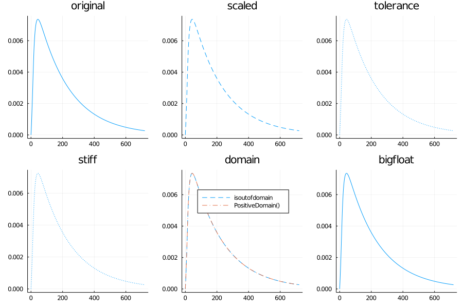
## Only scaling or increasing tolerance solves the issue
plot(layout=(2,3), size=(900,600))
plot!(sol_mtk_timepoint_original.t, label_frac_org, title="original",lab="", subplot=1)
plot!(sol_mtk_timepoint_scaled.t, label_frac_scaled, line=:dash, title="scaled",lab="",subplot=2)
plot!(sol_mtk_timepoint_tol.t, label_frac_tol, line=:dot, title="tolerance",lab="",subplot=3)
plot!(sol_mtk_timepoint_stiff.t, label_frac_stiff, line=:dot, title="stiff",lab="",subplot=4)
plot!(sol_mtk_timepoint_is.t, label_frac_is, line=:dash, title="domain",lab="isoutofdomain",subplot=5)
plot!(sol_mtk_timepoint_cb.t, label_frac_cb, line=:dashdot,lab="PositiveDomain()",subplot=5)
plot!(sol_mtk_timepoint_big.t, label_frac_big, title="bigfloat",lab="",subplot=6)
savefig(abspath(@__DIR__, "instability.pdf"))

## isoutofdomain or PositiveDomain don't seem to work
minimum(Matrix(VectorOfArray(sol_mtk_timepoint_is.u))[2,:])
minimum(Matrix(VectorOfArray(sol_mtk_timepoint_cb.u))[2,:])
minimum(Matrix(VectorOfArray(sol_mtk_timepoint_stiff.u))[2,:])
minimum(Matrix(VectorOfArray(sol_mtk_timepoint_tol.u))[2,:])
minimum(Matrix(VectorOfArray(sol_mtk_timepoint_scaled.u))[2,:])



## rerun model with da >> pa
d_a = 0.9
p_a = 0.005

p_da_big = [p_a,d_a]

ODE_mtk_model_da_big = ODEProblem(f_opt, u0,ts_num,p_da_big)

prob_da_big = remake(ODE_mtk_model_da_big, u0=u0_scaled)
prob_da_big_bigfloat = remake(ODE_mtk_model_da_big, u0=u0_big)


sol_mtk_timepoint_original = solve(ODE_mtk_model_da_big, Tsit5();saveat=ts_exp)
sol_mtk_timepoint_scaled = solve(prob_da_big, Tsit5();saveat=ts_exp)
sol_mtk_timepoint_is = solve(ODE_mtk_model_da_big, Tsit5();saveat=ts_exp, isoutofdomain=(y,p,t)->any(x->x<0,y))
sol_mtk_timepoint_cb = solve(ODE_mtk_model_da_big, Tsit5();saveat=ts_exp, callback=PositiveDomain())
sol_mtk_timepoint_tol = solve(ODE_mtk_model_da_big, Tsit5();saveat=ts_exp,abstol=1e-8,reltol=1e-8)
sol_mtk_timepoint_stiff = solve(ODE_mtk_model_da_big, Rodas5();saveat=ts_exp)
sol_mtk_timepoint_big = solve(prob_da_big_bigfloat, Tsit5();saveat=ts_exp)


label_frac_org = calc_label_frac(sol_mtk_timepoint_original)
label_frac_scaled = calc_label_frac(sol_mtk_timepoint_scaled)
label_frac_is = calc_label_frac(sol_mtk_timepoint_is)
label_frac_cb = calc_label_frac(sol_mtk_timepoint_cb)
label_frac_tol = calc_label_frac(sol_mtk_timepoint_tol)
label_frac_stiff = calc_label_frac(sol_mtk_timepoint_stiff)
label_frac_big = calc_label_frac(sol_mtk_timepoint_big)

plot(layout=(2,3), size=(900,600))
plot!(sol_mtk_timepoint_original.t, label_frac_org, title="original",lab="", subplot=1)
plot!(sol_mtk_timepoint_scaled.t, label_frac_scaled, line=:dash, title="scaled",lab="",subplot=2)
plot!(sol_mtk_timepoint_tol.t, label_frac_tol, line=:dot, title="tolerance",lab="",subplot=3)
plot!(sol_mtk_timepoint_stiff.t, label_frac_stiff, line=:dot, title="stiff",lab="",subplot=4)
plot!(sol_mtk_timepoint_is.t, label_frac_is, line=:dash, title="domain",lab="isoutofdomain",subplot=5)
plot!(sol_mtk_timepoint_cb.t, label_frac_cb, line=:dashdot,lab="PositiveDomain()",subplot=5)
plot!(sol_mtk_timepoint_big.t, label_frac_big, title="bigfloat",lab="",subplot=6)
savefig(abspath(@__DIR__, "instability_big_da.pdf"))



## Indentifying possible numerical instabilities

U_smooth(label_p[1:3], 720, label_p[4]) ## solution at latest time is around 1e-26

[ChrisRackauckas]

I have also tried using the PositiveDomain callback and isoutofdomain functions but both are not able to strictly enforces a positive solution for u2

Is it an instability or does the solution actually go negative?

[jonasmac16]

If you mean, if the system can actually become negative, then no. The solution should not become negative as it dependent u1 and U, which both should only reuturn positive values.

[devmotion]

It's not obvious to me that U_smooth would always return non-negative values since tanh (and hence h and h_inv) could potentially return negative values. However, if U could become negative, then du[2] is not guaranteed to be non-negative anymore.

[jonasmac16]

U_smooth is tending towards 0 with bigger t. Regardless, for the period we are solving for the smallest value of U_smooth is minimum([U_smooth(label_p[1:3], ts_exp[i], label_p[4]) for i in 1:721])=1.3857094869878607e-26, which is still positive.

[devmotion]

If it's problematic to solve the ODE in the original space and you've already tried isoutofdomain and PositiveDomain without success, my initial guess would be to perform the computations in log space instead. The resulting ODE system seems to be quite nice (mathematically), so maybe you can avoid the problems by using the model

function model(dv, v, p, t)
	@unpack pa, da, label = p
	c = 3.5
	U = U_smooth(t, label)
	dv[1] = pa - da
	dv[2] = -da + pa * c * U * exp(v[1] - v[2])
	return
end

where v[1] = log(u[1]) and v[2] = log(u[2]).

[devmotion]

BTW since U_smooth tends to zero and is quite small according to your comment above, it might be beneficial if you evaluate it in log space as well and use exp(logU + v[1] - v[2]) instead of U * exp(v[1] - v[2]).

[devmotion]

I just saw that actually your initial value for u[2] is zero, so you might want to transform only u[1] (initially).

[devmotion]

BTW it seems you can even completely decouple the ODEs by modelling v[2] = u[2] / u[1] directly (instead of u[2]) since dv[2] = pa * (c * U - v[2]).

[jonasmac16]

Thanks, I will try out your suggestions and see if they solve the problem more generally rather then scaling.

[devmotion]

I just quickly checked and only modelling the ratio u[1] / u[2] directly by dv[1] = pa * (c * U - v[2]) yields the following plots for the final parameter configuration:

It seems that's much more stable if you're interested in this particular quantity.

[jonasmac16]

Great, do you mind sharing the MWE. I think it will however be problematic for the actual model which has similar pairs of state variable e.g. u3 and u4 but both will be 0 at t=0. Thus, I was modelling them separately and only calculate the ratio for the observed times which are non-zero.

[devmotion]

I just replaced your model with

function U_smooth(t, fr, delta, beta, tau)
    a = tanh(5 * (t - tau))
    return exp(-delta * t) * (beta - fr) + fr * ((a + 1) * exp(-delta*(t - tau)) + (1 - a)) / 2
end

function model(du,u,p,t)
    pa, da, fr, delta, beta, tau = p
    c = 3.5

    U = U_smooth(t, fr, delta, beta, tau)

    du[1] = pa * (c * U - u[1])  # lA / A
	return
end

## simulation time range
tstep = 1.0
t_last = 720.0

ts_exp = collect(range(0.0,t_last;step=tstep))
ts_num = (0.0, t_last)

## kinetic parameters and initial conditions
da = 0.03
pa = 0.005
p = [pa, da, 0.0269266, 0.0788948, 0.0104485, 14.0]

u0 = [0.0]

## Setup model and use MTK to optimise code(this would also be done for the full model)
ODE_model = ODEProblem(model, u0, ts_num, p)

mtk_model= modelingtoolkitize(ODE_model)
f_opt = ODEFunction(mtk_model..., jac=true)
ODE_mtk_model = ODEProblem(f_opt, u0, ts_num, p)
....

and so on.

In general, I'm not sure if you can expect any "nice" dynamics of the ratio if it is not defined at the initial time point? Does it not even exist in the limit as t approaches 0?

[jonasmac16]

Thanks. I suppose it would be 0. With a limit what would one be able to do?

Also the other observable of the model is u1 itself hence I was modelling it explicitly.

[devmotion]

With a limit what would one be able to do?

I would assume you could use it as a proper initial value.

Also the other observable of the model is u1 itself hence I was modelling it explicitly.

I just removed it in my code since the instability seemed to be apparent mainly when evaluating the ratio, which I tried to model directly. You could just add it back to the ODE if you're interested in u1 as well.