Validation and training results Quantum Transfer Learning notebook

[AlexanderGeng]

Issue description

Qiskit Software	Version
qiskit-terra	0.18.3
qiskit-aer	0.9.0
qiskit-ignis	0.6.0
qiskit-ibmq-provider	0.16.0
qiskit-aqua	0.9.5
qiskit	0.30.1

Python	3.7.11 (default, Jul 27 2021, 14:32:16) [GCC 7.5.0]
OS	Linux
CPUs	12
Memory (Gb)	62.85524368286133
Fri Feb 18 18:53:45 2022 CET

And the newest versions of Pennylane.

Hello,

I tried the Quantum transfer learning notebook for my own dataset. Everything works quite fine and I get good classification results. However, two things are unclear to me:

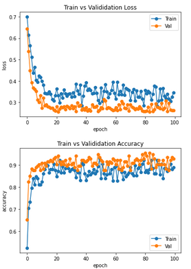
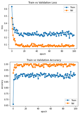
1. I have additionally recorded the losses and accuracies of Train and Val/Test dataset. So what is always output during training. Classically one expects there in the ideal case an exponential behavior, where the curves of Val/Test are worse than those of the training data set. That is, the loss curve of train should be below that of val/test and the accuracy curve above it. In my case, however, exactly the opposite is the case. At first I thought that perhaps my dataset is not well weighted, but this relationship also occurs in the classification of ants and bees in the notebook. What is the cause of this? This contradicts what I am used to from classical machine learning

2. Some days ago I had problems with the execution on real backends (see https://github.com/PennyLaneAI/qml/issues/426). The solution was updating pennylane-qiskit. However, if I try it also on the qasm_simulator via dev = qml.device('qiskit.aer', wires=n_qubits, backend='qasm_simulator'), the execution time is quite large compared to pennylane's default dev=qml.device('default.qubit', wires=n_qubits). It takes approximately 83 minutes to train 100 epochs and 900 images (default) and 2656 minutes for only 30 epochs using qasm_simulator. Is this a known problem or what is the reason for these differences?

[josh146]

It takes approximately 83 minutes to train 100 epochs and 900 images (default) and 2656 minutes for only 30 epochs using qasm_simulator. Is this a known problem or what is the reason for these differences?

Hi @Alex-259! My best guess for what is happening here is that default.qubit is optimized for gradient evaluation. That is, default.qubit by default will make use of backpropagation to compute gradients of variational circuits. With backpropagation, the gradient is extracted with only a constant memory overhead compared to the forward pass execution.

On the other hand, qasm_simulator is not optimized for quantum gradients, and therefore will fall back to the parameter-shift rule. The parameter-shift rule requires an additional 2p evaluations for p parameters to compute the gradient, so as you can see scales significantly worse compared to backpropagation!

For more details, check out our backprop vs. parameter-shift demonstration.

[AlexanderGeng]

Hi @josh146,

thanks for the quick and very good reply to my second point. That makes a big difference then of course. I have now run the Quantum Transfer Learning notebook with default.qubit and @qml.qnode(dev, interface='torch', diff_method="parameter-shift") for the 30 epochs for comparison. It takes there approximately 160 minutes. Thus, nearly 16 times faster than with qasm_simulator. Is this then due to the conversion from pennylane to qiskit or are there any other optimizations using default.qubit?

[CatalinaAlbornoz]

Hi @Alex-259, maybe you can try converting your circuit to qasm and running it in the IBM Quantum Lab. If it takes less time than your current time then there might be a conversion issue. If not then it may be something else. Please let us know what time you get so that we can dig deeper into this issue.

You can convert to qasm using dev._circuit.qasm(formatted=True) as shown in the second comment here. You can also export to qasm from the Tape of the qnode as shown in the second comment here.

I hope this helps and please let us know how much time it takes!

[AlexanderGeng]

Hi @CatalinaAlbornoz ,

thanks for your answer. I tested the differences for a very simple example. Since I also installed qiskit locally, I created one notebook with every test in it (comparable execution time results):

The results are the following:

default.qubit

start_time = time.time()
dev = qml.device("default.qubit", wires=2)
@qml.qnode(dev)
def circuit(param):
    qml.RX(param, wires=0)
    qml.RY(param, wires=1)
    qml.CNOT(wires=[0, 1])
    return qml.expval(qml.PauliZ(0)), qml.expval(qml.PauliZ(1))
print(circuit(np.pi / 5))
print("--- %s seconds ---" % (time.time() - start_time))

This gives the output

[0.80901699 0.6545085 ]
--- 0.09051513671875 seconds ---

qiskit.aer

start_time = time.time()
dev = qml.device("qiskit.aer", wires=2)
@qml.qnode(dev)
def circuit(param):
    qml.RX(param, wires=0)
    qml.RY(param, wires=1)
    qml.CNOT(wires=[0, 1])
    return qml.expval(qml.PauliZ(0)), qml.expval(qml.PauliZ(1))
print(circuit(np.pi / 5))
print("--- %s seconds ---" % (time.time() - start_time))

This gives the output

[0.81640625 0.70117188]
--- 2.5217936038970947 seconds ---

circuit converted to qasm_string

qasm_string=dev._circuit.qasm()
start_time = time.time()
qc = QuantumCircuit.from_qasm_str(qasm_string)
backend_sim = Aer.get_backend('qasm_simulator')
numOfShots = 1024
result_sim = execute(qc, backend_sim, shots=numOfShots).result()
counts_sim = result_sim.get_counts(qc)
print(counts_sim)
print("--- %s seconds ---" % (time.time() - start_time))

This gives the output

{'01': 14, '00': 865, '10': 71, '11': 74}
--- 0.07076907157897949 seconds ---

So, with qiskit.aer the execution time is ~28 times higher. Using the qasm_string the execution time is approximately the same as default.qubit. So, is it advisable to convert all circuits first to qiskit directly and then execute it there?

One additional question: Is there a clever way to get the expectation values as in pennylane qml.expval(qml.PauliZ(0)), qml.expval(qml.PauliZ(1)) also when using qiskit with the qasm_string (conversion from counts to the expectation values)? Or how this is solved with the qiskit.aer setting? I haven't found any code to it.

[AlexanderGeng]

Hi @co9olguy

thanks for the answer. Yes I see the point of the backpropagation vs. the parameter-shift-rule. Thanks a lot for your great efforts. However, I wonder if there are additional things that speed up the calculation in default.qubit that are not given in qiskit.aer. For me it seems that there are more optimizations inside, since also with default.qubit and diff_method="parameter-shift", I have less execution itme. But maybe this is the reason.

To my second question of my first post here: Has this ever happened to any of you that the values for loss/accuracy of training and validation do not match? That is, that the training provided larger loss and smaller accuracy values than the validation? Or does anyone have any ideas what I can do about it? I have checked and even remixed the data several times. It always shows similar curves as in my first post here.

[co9olguy]

Hi @Alex-259,

Unfortunately, I can't speculate too much, there could be many reasons. But obviously we've put a lot of energy and focus into making sure our default simulator works smoothly and efficiently within the library (since so many people end up using that). Definitely we have not put in as much effort making sure all plugins are working just as smoothly. So it could be something at the interface of PennyLane and the particular plugin (in this case Qiskit), it could be something in the underlying plugin (hard to know, out of our control), or it could just be that default.qubit is being built in alignment with the rest of PennyLane, so it naturally has a sort of implicit (if unintended) advantage over external plugins.

As for the second question, it does seem unusual. You'd expect the training loss to be lower than the validation loss. If I happened upon such a discrepency, I'd suspect a bug somewhere in the implementation. Beyond that, I'm not sure I can be of much help :slightly_smiling_face:

[AlexanderGeng]

Hey @co9olguy,

thanks for your answer. Yeah, I tested a lot to circumvent the unusual behavior between the training and validation loss/accuracy. But up to now, nothing results in the normal curves, where training is better than validation (lower loss, higher accuracy). What I have tried:

• Look if the dataset for validation is much simpler than that for training (is not the case)
• Change the splitting between training, validation, and test dataset
• Also change the ratio for splitting
• Change to some standard, not custom dataset (used also bee and ants as in the example)
• Exchange the linear layer with PCA

[angusjlowe]

Hi @Alex-259,

I just confirmed that even if you switch the training and validation datasets in this tutorial, you still get higher validation accuracy. It is possible that there is a bug in how these values are being computed, since as you mentioned this is not the expected behaviour. However, I also noticed that if you do not call model.eval() then this anomalous behaviour goes away -- perhaps there is a layer in the pretrained model that behaves differently depending on which mode (training/eval) is set?

[AlexanderGeng]

Hi @angusjlowe

thanks for your answer. Yes, it is a little bit weird, why this happens. What is different when using model.train() and model.eval() are the batch normalization layers:

• model.train(): Batchnorm layer calculates the batchwise mean and variance of the input and uses it to normalize the inputs
• model.eval(): Batchnorm doesn’t calculate the mean and variance of the input, but uses the pre-computed ones of the training stage

But I saw, validation is also better than training in the classical version when trained on the hymenoptera dataset https://pytorch.org/tutorials/beginner/transfer_learning_tutorial.html

Hard to figure out what's the exact reason for it

[CatalinaAlbornoz]

It's curious that the classical version shows the same behaviour. Thanks for pointing this out @Alex-259.

[andreamari]

Hi everyone,

As correctly pointed out by @angusjlowe, even in the PyTorch classical tutorial on transfer learning the training loss is smaller than the validation loss.

If I am not wrong, the reason is that the plotted loss is actually a running average over all instantaneous losses evaluated for each batch of data. This means that the training loss is the mean of bad contributions (loss of initial non-optimized batches) and good contributions (loss of final optimized batches). The validation loss is instead the running average of contributions which are all good since associated with optimized batches.

Maybe using a running average in this setting is not a good practice but has its own advantages (small fluctuations).

[CatalinaAlbornoz]

Thank you for your insight @andreamari!

[KetpuntoG]

Since the classical implementation fails in the same situation, it has been considered not to modify the demo. If necessary, we will reopen the issue again 🙂